Mock Final Examination

Question 1

What are the key components of financial losses essential for managing risk in general insurance, particularly concerning short-term products and the occurrence of insured events, and how do insurers analyze these components to optimize resource allocation and risk management strategies?

Solution to Question 1

Click to toggle answer

1. The key components of financial losses crucial for managing risk in general insurance, especially for short-term products, are the frequency and severity of claims.

2. Insurers analyze the likelihood of policyholders filing claims within a specified period through probability analysis, leveraging historical data and statistical methodologies.

Probability theory aids in evaluating the potential magnitude of individual claims, known as claim severity, by modeling the distribution of claim sizes and employing probabilistic techniques.

By understanding the frequency and severity of claims, insurers can optimize resource allocation and risk management strategies, fostering prudent financial planning and mitigation of adverse outcomes.

Question 2

What specific goals does employing probability tools in general insurance serve?

Solution to Question 2

Click to toggle answer

1. Probability analysis in general insurance facilitates the determination of insurance premiums by assessing risk probabilities, allowing insurers to customize premiums based on the anticipated frequency and severity of claims.

2. Actuarial models incorporate assessed risk probabilities to ensure a balance between affordability for policyholders and the financial sustainability of the insurance provider when determining premiums.

3. Probability theory guides insurers in creating reserves to serve as financial safeguards for future claim payments, enabling them to prudently allocate reserves based on assessed uncertainty linked with forthcoming claim liabilities.

4. The application of probability tools in general insurance ensures financial stability by meeting contractual obligations to policyholders over time through prudent reserve determination.

5. The application of probability tools in general insurance facilitates the development of risk management strategies aimed at mitigating adverse outcomes.

6. Probability tools in general insurance enhance decision-making processes related to underwriting and claims management, thereby optimizing resource allocation and improving overall operational efficiency.

Question 3

How can the method of moments be applied to estimate the parameters of a probability distribution for the number of daily claims using the provided data set?

3	5	2	4	6
7	8	4	3	5
6	9	10	3	5
2	4	6	7	8
4	3	5	6	9

Solution to Question 3

Click to toggle answer

Let us apply the method of moments to estimate the parameters of a probability distribution for the number of daily claims using the provided data set.

Given Data Set:

3	5	2	4	6
7	8	4	3	5
6	9	10	3	5
2	4	6	7	8
4	3	5	6	9

1. Calculate the sample moments: Mean (first moment):

\[\bar{X} = \frac{1}{n} \sum_{i=1}^{n} X_i\]

\[\bar{X} = \frac{3+5+2+...+9}{25} = 5.36\]

Variance (second central moment):

\[S^2 = \frac{1}{n-1} \sum_{i=1}^{n} (X_i - \bar{X})^2\]

\[S^2 = \frac{(3-5.04)^2 + (5-5.04)^2 + ... + (9-5.04)^2}{24} = 5.07\]

2. Choose a probability distribution to fit to the data. Let’s assume the number of daily claims follows a Poisson distribution.

The mean of a Poisson distribution is denoted by (\(\lambda\)). Consequently, we equate the sample mean to the theoretical mean of the Poisson distribution:

Mean: \(\lambda = 5.36\)

Therefore, the estimated parameter (\(\lambda\)) for the Poisson distribution representing the number of daily claims is approximately 5.36.

This process provides an estimate of the parameter of the Poisson distribution that best fits the given data set.

Exploring Poisson Distribution Fitting with Method of Moments in R

In this exploration, we illusrtate how to fit a Poisson distribution to a set of daily claims data using the Method of Moments in R.

The provided R code showcases key steps including

• data summary,

• visualization,

• parameter estimation,

• PMF calculation, and

• plotting.

The explanation below guides through each step, elucidating the process of fitting the distribution and comparing it with the observed data. Let us dive into the code and understand how the Method of Moments is employed to estimate the parameters of the Poisson distribution and visualize its fit to the data.

Code explanation

• Data Summary: The initial step involves summarizing the provided daily claims data by computing its sample mean and variance.

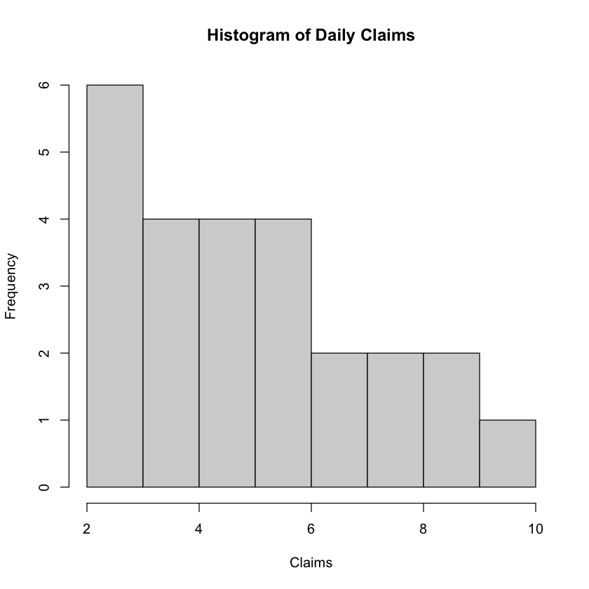
• Visualization: To gain insights into the distribution of the data, a histogram is created, displaying the frequency distribution of the daily claims.

• Parameter Estimation: Employing the Method of Moments, an estimation of the parameter lambda for the Poisson distribution is made, using the sample mean as its estimate.

• Probability Mass Function (PMF): A PMF function for the Poisson distribution is defined to calculate the probability of observing a specific number of claims.

• PMF Calculation: Using the estimated lambda and a range of claim values, the PMF values for the fitted Poisson distribution are computed.

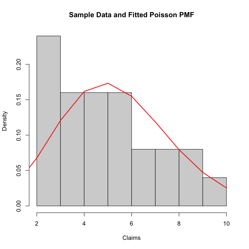
• Plotting: The sample histogram is plotted again, this time without frequencies, and the PMF curve for the fitted Poisson distribution is superimposed on it. This allows for visual comparison between the observed data and the fitted distribution.

Show code cell source Hide code cell source

claims <- c(3, 5, 2, 4, 6, 7, 8, 4, 3, 5, 6, 9, 10, 3, 5, 2, 4, 6, 7, 8, 4, 3, 5, 6, 9)

# Sample mean
mean_claims <- mean(claims)
cat("Sample mean:", mean_claims, "\n")

# Sample variance
var_claims <- var(claims)
cat("Sample variance:", var_claims, "\n")

# Visualize data
hist(claims, breaks = 10, main = "Histogram of Daily Claims", xlab = "Claims")


# Method of Moments estimation for lambda
lambda_mm <- mean_claims
cat("Method of Moments estimation for lambda:", lambda_mm, "\n")

# PMF function for Poisson distribution
pmf_poisson <- function(x, lambda) {
  return(dpois(x, lambda))
}

# Generate x values for PMF
x_values <- 0:max(claims)

# Calculate PMF for fitted Poisson distribution
pmf_values <- pmf_poisson(x_values, lambda_mm)

# Plot sample histogram
hist(claims, breaks = 10, main = "Sample Data and Fitted Poisson PMF", xlab = "Claims", freq = FALSE)

# Superimpose PMF on histogram
lines(x_values, pmf_values, type = "l", col = "red", lwd = 2)

Sample mean: 5.36 

Sample variance: 5.073333 

Method of Moments estimation for lambda: 5.36 

Notes: Leveraging Fitted Poisson Distribution for Probability Questions

Click to toggle notes

Given that the Poisson distribution provides a satisfactory fit to the sample daily claim numbers dataset, how can we use the fitted model to address probability questions?

Consider questions such as:

1. What is the anticipated number of daily claims?

2. What is the probability that the daily claims number will surpass 10?

Exploring these questions involves leveraging the fitted Poisson distribution to estimate probabilities and make informed decisions based on the data.

The R code below shows how we can use the fitted model to tackle such probability questions.

Show code cell source Hide code cell source

# Fitted lambda value from Method of Moments estimation
lambda_mm <- mean_claims  # Assuming lambda is estimated using Method of Moments

# (1) Expected number of daily claims
expected_claims <- lambda_mm
cat("Expected number of daily claims:", expected_claims, "\n")

# (2) Probability of daily claims exceeding 10
prob_exceed_10 <- 1 - ppois(10, lambda_mm)
cat("Probability of daily claims exceeding 10:", prob_exceed_10, "\n")

Expected number of daily claims: 5.36 

Probability of daily claims exceeding 10: 0.02148183 

Notes: Limitations of Using Only Sample Data for Probability Questions

Click to toggle notes

Limitations of Using Only Sample Data for Probability Questions

Using only the sample daily claims data without fitting a model, such as the Poisson distribution, presents limitations in answering probability questions directly. Here’s why:

1. Expected Number of Daily Claims: Without fitting a distribution model, determining the expected number of daily claims becomes challenging. While the sample mean provides an estimate, it might not accurately represent the underlying distribution. Variability in the data might exist, making the sample mean less reliable as a predictor of future claims.

2. Probability of Exceeding a Certain Number of Claims: Calculating the probability of exceeding a specific number of claims without a fitted model involves making assumptions about the underlying distribution. For instance, one might assume a normal distribution and calculate probabilities based on mean and standard deviation. However, if the data does not follow a normal distribution, these probabilities might be inaccurate.

In summary, while basic statistics from the sample data like mean and variance offer insights, they might not suffice for precise probability calculations. Utilizing a fitted distribution model, such as the Poisson distribution in this case, provides a more robust framework for addressing probability questions and making informed decisions based on the data’s underlying distribution.

Question 4

What implications arise when the sample mean and variance of a dataset significantly differ when applying the method of moments to estimate parameters specifically for a Poisson distribution?

Solution to Question 4

Click to toggle answer

When the sample mean and variance of a dataset significantly differ, it suggests that the data may not match the Poisson distribution, where the mean and variance are equal.

This discrepancy indicates a potential mismatch between the assumed Poisson distribution and the actual characteristics of the data. Consequently, alternative distributions with separate parameters for mean and variance or different shapes may be more suitable for modeling.

Additionally, further exploration of the data and consultation with domain experts may be necessary to understand underlying patterns and select an appropriate distribution for accurate estimation.

Question 5

How can the method of moments be employed to estimate the parameters of a probability distribution for the individual claims amounts using the provided data set of 100 individual claims?

1063.76	1077.21	877.98	1016.89	1096.54	1106.83	1257.81	866.99	1055.64	1080.94
1250.91	1077.39	844.44	1086.88	1171.13	968.36	1104.12	1068.82	1116.36	1035.07
951.28	856.52	922.12	1009.02	998.69	1137.45	1012.21	1230.22	983.76	991.36
887.74	1038.94	955.66	823.67	1144.09	1100.25	1057.96	1005.27	1015.41	799.31
938.18	1161.93	891.14	983.42	1101.29	974.55	1253.01	835.68	869.14	1093.06
1220.84	1051.88	1106.61	1071.09	1022.18	1065.24	983.89	1128.74	1133.64	1003.42
905.89	1044.67	1031.41	1016.04	858.35	977.67	983.48	962.29	1025.42	1020.88
1042.97	833.07	873.13	1068.19	1046.24	1128.57	1148.35	938.06	1040.09	1040.72
1102.64	904.82	967.89	1112.22	960.01	883.34	1263.42	1185.6	1165.66	990.54
1200.24	872.72	921.81	1116.09	961.53	1154.97	1028.86	986.72	1093.95	1043.34

Solution to Question 5

Click to toggle answer

To fit the individual claims amounts dataset using the Method of Moments, we first compute the sample mean (\(\bar{x}\)) and sample variance \((s^2\)) of the dataset. In this case, the sample mean is calculated to be approximately 1029.358 and the sample variance is approximately 11535.67.

Next, we employ the Method of Moments to estimate the parameters of the normal distribution, namely the mean (\(\mu\)) and standard deviation (\(\sigma\)), using the sample mean and variance. The sample mean is used as the estimate for the population mean (\(\mu\)), and the square root of the sample variance is used as the estimate for the population standard deviation (\(\sigma\)).

The formula for the sample mean (\(\bar{x}\)) is:

\[ \bar{x} = \frac{1}{n} \sum_{i=1}^{n} x_i \]

where \(x_i\) is the \(i\)th observation in the dataset and \(n\) is the total number of observations.

The formula for the sample variance (\(s^2\)) is:

\[ s^2 = \frac{1}{n-1} \sum_{i=1}^{n} (x_i - \bar{x})^2 \]

where \(x_i\) is the \(i\)th observation in the dataset, \(\bar{x}\) is the sample mean, and \(n\) is the total number of observations.

The estimated parameters of the normal distribution, derived through the Method of Moments using the sample mean (\(\bar{x}\)) and sample variance (\(s^2\)) of the individual claims amounts dataset, are approximately 1029.358 and 11535.67, respectively.

By utilizing the Method of Moments, we obtain estimates for the parameters of the normal distribution that best describe the dataset’s distribution. These estimated parameters allow us to model the dataset using a normal distribution, providing insights into the underlying distribution of the individual claims amounts.

Exploring Normal Distribution Fitting with Method of Moments in R

In this exploration, we illusrtate how the Method of Moments be employed to estimate the parameters of a probability distribution for the individual claims amounts using the provided dataset of 100 individual claims.

Let us explore fitting a normal distribution to the data and understand how the Method of Moments can help estimate its parameters.

Explanation of Main Steps

1. Data Initialization: Initialize a vector claims with the provided individual claims amounts dataset.

2. Sample Mean and Variance Calculation: Compute the sample mean and variance of the claims data.

3. Parameter Estimation: Use the Method of Moments to estimate the parameters of the normal distribution, namely the mean (μ) and standard deviation (σ), using the sample mean and variance.

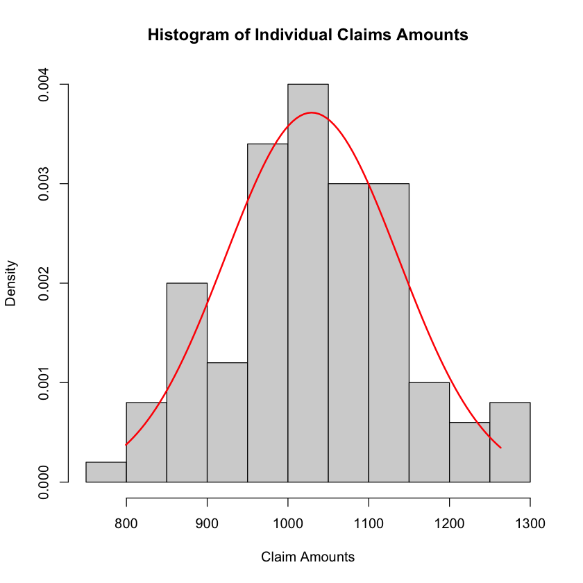
4. PDF Function Definition: Define a function pdf_normal to calculate the Probability Density Function (PDF) of the normal distribution.

5. Comparison Between Fitted Model and Sample Data: Generate x values for the PDF of the fitted normal distribution and calculate the PDF values. Then, plot the sample histogram of claim amounts along with the PDF curve for the fitted normal distribution to visually compare the distribution of the sample data with the fitted model.

Show code cell source Hide code cell source

# Initialize claims data
claims <- c(
  1063.76, 1077.21, 877.98, 1016.89, 1096.54,
  1106.83, 1257.81, 866.99, 1055.64, 1080.94,
  1250.91, 1077.39, 844.44, 1086.88, 1171.13,
  968.36, 1104.12, 1068.82, 1116.36, 1035.07,
  951.28, 856.52, 922.12, 1009.02, 998.69,
  1137.45, 1012.21, 1230.22, 983.76, 991.36,
  887.74, 1038.94, 955.66, 823.67, 1144.09,
  1100.25, 1057.96, 1005.27, 1015.41, 799.31,
  938.18, 1161.93, 891.14, 983.42, 1101.29,
  974.55, 1253.01, 835.68, 869.14, 1093.06,
  1220.84, 1051.88, 1106.61, 1071.09, 1022.18,
  1065.24, 983.89, 1128.74, 1133.64, 1003.42,
  905.89, 1044.67, 1031.41, 1016.04, 858.35,
  977.67, 983.48, 962.29, 1025.42, 1020.88,
  1042.97, 833.07, 873.13, 1068.19, 1046.24,
  1128.57, 1148.35, 938.06, 1040.09, 1040.72,
  1102.64, 904.82, 967.89, 1112.22, 960.01,
  883.34, 1263.42, 1185.60, 1165.66, 990.54,
  1200.24, 872.72, 921.81, 1116.09, 961.53,
  1154.97, 1028.86, 986.72, 1093.95, 1043.34
)

# Sample mean and variance calculation
mean_claims <- mean(claims)
var_claims <- var(claims)

# Print sample mean and sample variance
cat("Sample Mean:", mean_claims, "\n")
cat("Sample Variance:", var_claims, "\n")

# Parameter estimation using Method of Moments
mu_mm <- mean_claims
sigma_mm <- sqrt(var_claims)

# PDF function for Normal distribution
pdf_normal <- function(x, mean, sd) {
  return(dnorm(x, mean, sd))
}

# Generate x values for PDF
x_values <- seq(min(claims), max(claims), length.out = 100)

# Calculate PDF for fitted Normal distribution
pdf_values <- pdf_normal(x_values, mu_mm, sigma_mm)

# Plotting
hist(claims, breaks = 10, freq = FALSE, main = "Histogram of Individual Claims Amounts", xlab = "Claim Amounts")
lines(x_values, pdf_values, type = "l", col = "red", lwd = 2)

Sample Mean: 1029.358 

Sample Variance: 11535.67 

Question 6

What formula can be used to compute the sample skewness, and what implications arise from the skewness obtained from analyzing the sample data?

Solution to Question 6

Click to toggle answer

To calculate the sample skewness, the following formula can be used:

\[\text{Sample Skewness} = \frac{1}{(n-1)\cdot S^3} \sum_{i=1}^{n} \left( X_i - \bar{X} \right)^3\]

Where:

• \( n \) is the number of observations.

• \( X_i \) is the \( i \)-th observation.

• \( \bar{X} \) is the sample mean.

• \( S \) is the sample standard deviation.

The skewness obtained from analyzing the sample data provides insights into the asymmetry of the distribution.

• A positive skewness indicates a right-skewed distribution, where the tail extends to the right and there are relatively more high values.

• Conversely, a negative skewness indicates a left-skewed distribution, with relatively more low values.

• A skewness close to zero suggests a symmetric distribution. Understanding the skewness helps in assessing the distribution’s shape and making informed decisions in various fields, such as finance, economics, and insurance.

From the calculated sample skewness of approximately 0.276, we can conclude that the distribution of individual claims amounts may exhibit a slight positive skewness.

Here’s what this conclusion implies:

1. Positive Skewness:

• A positive skewness suggests that the distribution may be slightly right-skewed.

• In the context of insurance claims, this indicates that there may be some high-value claims that are relatively higher than the average, leading to a distribution where the tail extends more to the right.

• Insurers should be aware of the possibility of occasional high-value claims and consider them when assessing risk and setting premiums.

2. Asymmetry:

• The positive skewness indicates that the distribution is not perfectly symmetric, meaning that there may be an imbalance between high and low values.

• Insurers may need to account for this asymmetry when conducting risk analysis and financial planning.

3. Magnitude:

• With a skewness of approximately 0.276, the positive skewness is relatively small, suggesting that the asymmetry in the distribution is not very pronounced.

• While there is some skewness present, it may not have a significant impact on risk assessment and premium calculation compared to distributions with larger skewness values.

In summary, the positive skewness of approximately 0.276 suggests a slight right-skew in the distribution of individual claims amounts. Insurers should consider this asymmetry when evaluating risk and making decisions related to pricing and risk management.

Question 7

What statistical methods and visualizations can be used to assess whether the distribution of individual claims amounts follows a normal distribution, and how can these approaches confirm or reject the hypothesis of normality?

Solution to Question 7

Click to toggle answer

To confirm whether the distribution of individual claims amounts follows a normal distribution, we can utilize various statistical tests and visualizations. Here are some approaches:

1. Normal Probability Plot (Q-Q Plot):

   • Plot the quantiles of the observed data against the quantiles of a normal distribution.

   • If the data points approximately fall along a straight line, it suggests that the data follows a normal distribution.

2. Histogram:

   • Create a histogram of the data and compare it visually to the bell-shaped curve of a normal distribution.

   • While not definitive, a symmetric and bell-shaped histogram is indicative of a normal distribution.

3. Shapiro-Wilk Test:

   • Perform the Shapiro-Wilk test for normality.

   • This test provides a p-value, and if it is greater than a chosen significance level (e.g., 0.05), it indicates that the data is normally distributed.

4. Kolmogorov-Smirnov Test:

   • Conduct the Kolmogorov-Smirnov test for normality.

   • This test compares the empirical cumulative distribution function of the data to the cumulative distribution function of a normal distribution.

   • If the test statistic is not significant at a chosen significance level, it suggests that the data is normally distributed.

5. Anderson-Darling Test:

   • Apply the Anderson-Darling test for normality.

   • This test evaluates whether the sample data comes from a specified distribution (in this case, a normal distribution).

   • If the resulting statistic is less than the critical value at a chosen significance level, it supports the hypothesis that the data is normally distributed. By employing these methods, we can confirm whether the distribution of individual claims amounts is approximately normal or if an alternative distribution might be more suitable. It’s essential to consider multiple approaches to ensure robustness in the assessment of distributional assumptions.

See https://datatab.net/tutorial/test-of-normality for more details.

Question 8

Insurance coverage for the standalone batteries of an electric vehicle (EV) encompasses various protections against risks and issues affecting the battery’s performance and longevity. This coverage aims to safeguard EV owners from financial burdens associated with battery-related problems, ensuring uninterrupted usage and peace of mind.

Can you describe the actuarial phenomena, events, frequency, severity, and timing in the context of insurance products covering the battery life of EV cars?

Solution to Question 8

Click to toggle answer

• Actuarial Phenomena: Actuarial phenomena in insurance products covering EV battery life encompass various occurrences impacting financial risks, including battery degradation, malfunctions, premature aging, and unexpected failures over time. Actuaries analyze historical data and predictive models to understand these phenomena’s frequency, severity, and financial implications for insurance companies.

• Events: In this context, events refer to incidents triggering coverage or claims under the insurance policy, such as battery degradation beyond a threshold, mechanical or electrical failures, or premature aging. These events occur progressively over the EV’s lifespan, leading to potential claims at various points in time.

• Frequency: Frequency denotes the rate of insurance claims within a given period, relating to how often insured events occur. Actuaries estimate the frequency of battery-related events over time, helping insurers determine appropriate premiums and reserves.

• Severity: Severity refers to the financial impact of an individual insurance claim, such as the cost of repairing or replacing a faulty battery. It varies based on the timing, extent of damage, and repair or replacement expenses incurred.

• Timing: Timing plays a critical role, as events unfold gradually over the EV’s lifespan. It involves understanding when events occur, how they progress, and their impact on the frequency and severity of insurance claims. Actuaries consider timing factors to develop risk models, pricing strategies, and claims management protocols.

Question 9

What are the specific methodologies and approaches used by insurance companies to address risks associated with EV battery performance, degradation, and potential failures? This discussion should encompass the processes of risk identification, assessment, and management, along with strategies aimed at mitigating negative impacts and leveraging positive outcomes.

Furthermore, how do insurance companies employ risk transfer mechanisms to mitigate the financial impact of these risks?

Solution to Question 9

Click to toggle answer

Insurance companies employ a multifaceted approach to address risks associated with EV battery performance, degradation, and potential failures.

1. Risk Identification:

   • To identify risks, insurance companies analyze various factors including battery age, usage patterns, environmental conditions, and technological limitations. This comprehensive assessment helps in understanding the potential threats to EV battery reliability and longevity.

2. Risk Assessment:

   • After identifying risks, insurance companies assess their likelihood and potential impact. This involves analyzing historical data, conducting predictive modeling, and consulting with experts to quantify the probability of battery-related issues occurring and their financial implications for the insurer.

3. Risk Management:

   • To effectively manage risks, insurance companies develop strategies such as offering maintenance guidelines to EV owners, incentivizing safe driving practices, and collaborating with manufacturers to improve battery design and quality control processes. These measures aim to prevent or minimize the occurrence and impact of battery-related issues.

4. Mitigation of Negative Impacts:

   • Insurance companies provide comprehensive coverage for battery repairs, replacements, and related expenses to mitigate the negative impacts of battery failures or degradation beyond normal wear and tear. This ensures that EV owners are financially protected in case of unforeseen battery-related issues.

5. Risk Transfer Mechanisms:

   • In addition to internal risk management strategies, insurance companies utilize risk transfer mechanisms such as reinsurance or securitization to spread or mitigate the financial impact of large-scale battery failures or claims. This helps maintain the insurer’s financial stability and ensures the fulfillment of obligations to policyholders in the event of significant losses related to EV battery issues. Overall, insurance companies employ a combination of risk identification, assessment, and management processes, alongside strategies for mitigating negative impacts and utilizing risk transfer mechanisms, to effectively address risks associated with EV battery performance, degradation, and potential failures.

Question 10

Crop insurance products play a crucial role in safeguarding farmers’ livelihoods and mitigating financial risks associated with agricultural activities. These insurance products provide protection against various perils such as adverse weather conditions, pest infestations, and market fluctuations, ensuring that farmers can recover financially from crop-related losses and continue their farming operations.

How do insurance companies manage risks associated with crop insurance products, encompassing risk identification, assessment, and management processes, alongside strategies for mitigating negative impacts and utilizing risk transfer mechanisms?

Solution to Question 10

Click to toggle answer

Insurance companies use a comprehensive approach to address risks associated with crop insurance products, which involves various key elements:

1. Risk Identification:

   • To identify risks, insurance companies analyze factors such as weather patterns, soil quality, pest infestations, and market fluctuations. By understanding these factors, insurers can assess the likelihood of crop-related losses and damage.

2. Risk Assessment:

   • After identifying risks, insurance companies assess their potential impact on crop yields and financial losses. This assessment may involve historical data analysis, crop modeling, and consultation with agronomists to estimate the probability of various risk events occurring and their potential severity.

3. Risk Management:

   • To manage risks effectively, insurance companies develop strategies such as offering customized insurance products tailored to specific crops, regions, and risk profiles. Additionally, insurers may provide risk mitigation services such as agronomic advice, crop monitoring, and access to crop insurance education programs for farmers.

4. Mitigation of Negative Impacts:

   • Insurance companies provide coverage for crop losses caused by adverse events such as droughts, floods, storms, pests, and diseases. This coverage helps farmers recover financially from crop-related losses, ensuring their livelihoods are protected and enabling them to continue farming operations.

5. Risk Transfer Mechanisms:

   • In addition to internal risk management strategies, insurance companies may utilize risk transfer mechanisms such as reinsurance or financial derivatives to mitigate their exposure to large-scale crop losses. These mechanisms help spread the financial risk among multiple parties and ensure the insurer’s ability to honor policyholder claims, even in the event of catastrophic crop failures.

Question 11

What is the role of an actuarial model in the insurance industry, and how do actuaries utilize these models to understand and manage risks effectively? Please provide examples to illustrate the application of actuarial models in risk management.

Solution to Question 11

Click to toggle answer

An actuarial model is a fundamental tool used by actuaries in the insurance industry to quantify and manage risks associated with insurance products.

These models use mathematical and statistical techniques to

• analyze historical data,

• predict future events, and

• assess the financial impact of various risk scenarios.

Actuarial models can be applied across different areas of insurance, including pricing, reserving, and underwriting, to help insurers make informed decisions and ensure their financial stability.

For example, in pricing insurance premiums, actuaries use actuarial models to estimate the expected claims costs based on factors such as policyholder demographics, historical loss experience, and market trends. By incorporating these factors into the model, insurers can accurately price their products to cover anticipated claims while remaining competitive in the market.

In reserving, actuarial models are used to estimate the amount of money insurers need to set aside to cover future claim payments. These models take into account factors such as the development of claims over time, the likelihood of claims being reported, and the severity of potential losses. By regularly updating reserves based on actuarial modeling results, insurers can ensure they have sufficient funds to meet their obligations to policyholders.

Similarly, actuarial models play a crucial role in underwriting decisions by assessing the risk profile of potential policyholders and determining appropriate coverage levels and premiums. These models analyze various risk factors, such as health status, driving behavior, or property characteristics, to evaluate the likelihood of claims and set pricing accordingly.

Overall, actuarial models serve as powerful tools for insurers to understand and manage risks effectively, enabling them to make data-driven decisions that support their financial stability and long-term success in the insurance market.

Question 12

What is the concept of the time value of money, and how does it impact financial decision-making?

Please provide an example to illustrate how the time value of money affects the value of cash flows over time.

Solution to Question 12

Click to toggle answer

The time value of money is a fundamental financial concept that states that a dollar today is worth more than a dollar in the future due to its potential earning capacity or interest-bearing potential over time.

This concept is based on the premise that money has the ability to earn interest or generate returns, and therefore, the value of money changes over time.

The time value of money affects financial decision-making in various ways, including investment analysis, loan pricing, and capital budgeting.

For example, when evaluating investment opportunities, investors consider the time value of money to determine the present value of future cash flows. By discounting future cash flows back to their present value using an appropriate discount rate, investors can compare the value of different investment options and make informed decisions about where to allocate their capital.

Example

The time value of money dictates that money available today is worth more than the same amount in the future due to its potential to earn interest or returns. For instance, $100 received today is more valuable than $100 received one year from now because the $100 received today can be invested and earn interest over the year, increasing its value.

Therefore, considering the time value of money is essential for making informed financial decisions regarding investments, loans, and capital budgeting.

Question 13

Derive the formula for calculating the future value of an annuity payable of 1 baht in arrears for n years. Additionally, illustrate the timeline representing the cash flows associated with this annuity.

Solution to Question 13

Click to toggle answer

Based on the first principles,

\[ \begin{align} s_{\overline{n|}} &= (1+i)^{n-1} + (1+i)^{n-2} + \ldots + (1+i) + 1. \end{align} \]

Multiplying the equation through by (1+i) gives

\[(1+i) \cdot s_{\overline{n|}} = (1+i)^{n} + (1+i)^{n-1} + \ldots + (1+i)^2 + (1+i).\]

Subtracting the two equations results in

\[\begin{split}\begin{aligned} i \cdot s_{\overline{n|}} &= (1+i)^{n} - 1\\ s_{\overline{n|}} &= \frac{(1+i)^{n} - 1}{i}.\end{aligned}\end{split}\]

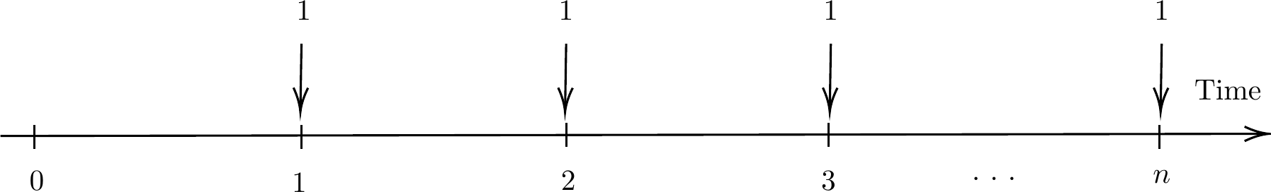
Fig. 22 A series of unit payments at the end of each year for \(n\) years

Question 14

Why is the loan amount \(L\) considered the present value of the regular level annual loan repayments \(P\) made over \(n\) years, calculated at an annual loan rate of \(i\%\)? Please explain the rationale behind this relationship.

Solution to Question 14

Click to toggle answer

The loan amount \(L\) is considered the present value of the regular level annual loan repayments \(P\) made over \(n\) years because it represents the current worth of future repayments discounted at the loan rate \(i\). This relationship is based on the time value of money, where cash flows in the future are worth less than those in the present due to the opportunity cost of not investing the funds. By discounting the future repayments to their present value, we account for this time value of money and determine the initial amount needed to cover the loan.

Consequently, it follows that

\[L = P \cdot a_{\overline{n|}i}.\]

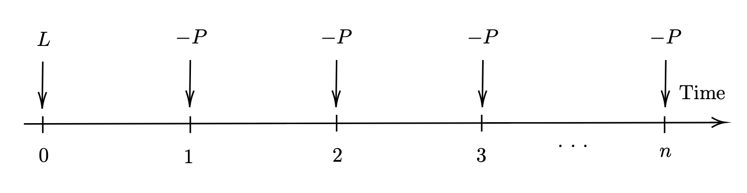
Fig. 23 The timeline of loan repayment

Question 15

How do regular level annual loan repayments \(P\) made over \(n\) years, calculated at an annual loan rate of \(i\%\), contribute to the repayment of a loan? Additionally, please construct a loan schedule illustrating the repayment process.

A loan schedule is a tabular representation detailing the repayment process of a loan over time. It typically includes columns for the period (e.g., year or month), the beginning loan balance, loan repayments, interest payments, principal payments, and the ending loan balance. The schedule provides a comprehensive overview of how the loan balance decreases over time as payments are made, demonstrating the repayment progress and the allocation of payments towards interest and principal.

Solution to Question 15

Click to toggle answer

A more general form of loan payments can be expressed as follows: Let

• \(L_t\) be the amount of the loan outstanding at time \(t\).

• \(X_t\) be the instalment at time \(t\) (all instalments may not be the same amount).

• \(i\) be the effective rate of interest per time unit charged on the loan.

  Time	Repayment	Interest content	Capital content	Capital outstanding
  \(0\)				\(L_0\)
  \(1\)	\(X_1\)	\(iL_0\)	\((X_1 - iL_0)\)	\(L_1 = L_0 - (X_1 - iL_0)\)
  \(2\)	\(X_2\)	\(iL_1\)	\((X_2 - iL_1)\)	\(L_2 = L_1 - (X_2 - iL_1)\)
  \(\vdots\)
  \(t\)	\(X_t\)	\(iL_{t-1}\)	\((X_t - iL_{t-1})\)	\(L_t = L_{t-1} - (X_t - iL_{t-1})\)
  \(\vdots\)
  \(n\)	\(X_n\)	\(iL_{n-1}\)	\((X_n - iL_{n-1})\)	0

Note The capital outstanding after the \(k\)th payment is \(P a_{\overline{n|}}\), which is the present value of future repayments. This holds even when the repayments and interest rates are not constant.

Example

You borrow ฿5,000 for a term of 3 years at a fixed interest rate of 10% pa. The loan is to be repaid by 3 level annual repayments of ฿2,010.57 at the end of each year. Calculate the interest content, capital content from each repayment and capital outstanding after such repayment.

The loan payments can be expressed in the form of a Loan Schedule as follows:

Time	Repayment	Intest content	Capital content	Capital outstanding
0				5000
1	2010.57	500	1510.57	3489.43
2	2010.57	348,943	1661.627	1827.80
3	2010.57	182.780	1827.79	0.01