2.3 Probability Distributions

2.3 Probability Distributions#

Random variables#

Random variables are fundamental in probability theory and statistics, representing numerical outcomes of random phenomena.

In actuarial science, a common example of a random variable is the number of insurance claims received by an insurance company within a certain period, such as a month, denoted as $X$ . This variable can take on different values depending on various factors such as the number of accidents, the severity of accidents, driving conditions, and so on. For example, in a particular month,

$X$ could be 0 if there are no accidents reported by policyholders.
It could be 1 if only one policyholder files a claim for a minor accident.
It could be 2 if there are two separate accidents reported, and so forth.

By defining the variable $X$ as the number of car insurance claims in a month, we have created a random variable that captures the variability and uncertainty inherent in the number of claims an insurance company might receive within a specific period.

This random variable is essential for actuarial calculations, such as estimating claim frequencies, setting premiums, and determining reserve requirements.

Definition

A random variable is a function that assigns a real number to each outcome in the sample space of a random experiment.

A random variable is like a translator between the real world and numbers. It takes things that can happen, like flipping a coin, and turns them into numbers we can work with.

For example, if we flip a coin, we could have a random variable called “X” that says “0” if it lands on tails and “1” if it lands on heads. So, instead of dealing with the actual outcomes, we use numbers to represent them, making it easier to do calculations and understand probabilities.

Example 2.31: Bernoulli random variable

In actuarial science, a common example of a Bernoulli random variable is whether an insurance policyholder makes a claim within a specified period, such as a month. Let us denote this Bernoulli random variable as $X$ .

For instance, consider a scenario where a policyholder either makes a claim ( $X = 1$ ) or does not make a claim ( $X = 0$ ) during a month. Here, $X$ represents the outcome of a single trial with two possible outcomes: success (making a claim) or failure (not making a claim). This setup fits the definition of a Bernoulli random variable, where the parameter $p$ represents the probability of success, i.e., the likelihood of a policyholder making a claim within the given period.

Here, $X$ is a discrete random variable that takes on the values 0 and 1.

By analyzing the distribution of $X$ , actuaries can estimate the probability of claim occurrence, crucial for pricing insurance policies, setting reserves, and assessing risk.

Example 2.32: An example of a continuous random variable

An example of a random variable representing waiting time for the next insurance claim in actuarial science can be denoted as $X$ . In this scenario, $X$ represents the time interval between consecutive insurance claims, measured in months, days, or any other appropriate unit.

For instance, suppose a policyholder submits a claim today, and we are interested in the time it takes until the next claim is received. Let us say $X = 0.5$ if a claim is made after half a month, $X = 1$ if it takes a month, $X = 2$ if it takes two months, and so forth.

Here, $X$ is a continuous random variable defined for all $X \geq 0$ , as waiting time cannot be negative. Actuaries analyze the distribution of $X$ to understand the frequency and patterns of claim occurrences over time, aiding in pricing insurance products, estimating reserve amounts, and managing risk.

Types of Random Variables#

There are mainly two types of random variables:

Discrete Random Variables
- Discrete random variables take on a countable number of distinct values.
- Examples include the number of customers in a queue, the number of defective items in a batch, or the outcome of rolling a die.
Continuous Random Variables
- Continuous random variables can take on any value within a given range or interval.
- They are associated with measurements and are often represented by real numbers.
- Examples include the height of a person, the time taken to complete a task, or the temperature of a room.

Probability functions#

Random variables are intimately connected with probability functions, which quantify the likelihood of different outcomes associated with those variables.

Discrete Random Variables#

Discrete random variables, representing outcomes with distinct values, are characterized by probability mass functions (PMFs), providing a systematic way to assign probabilities to each possible outcome.

Probability Mass Function (PMF)

The probability mass function (PMF), denoted as $f (x) = P (X = x)$ , provides the probability that a discrete random variable $X$ takes on a specific value $x$ . It assigns probabilities to each possible outcome of the random variable.

Cumulative Distribution Function (CDF)

The cumulative distribution function (CDF), denoted as $F (x)$ , calculates the probability that a discrete random variable $X$ is less than or equal to a given value $x$ . It sums up the probabilities from the PMF up to and including $x$ , providing a cumulative measure of the distribution. Hence,

F (x) = P (X \leq x) .

Continuous Random Variables#

Continuous random variables, on the other hand, are associated with probability density functions (PDFs), which describe the relative likelihood of the variable taking on different values within a continuous range.

Probability Density Function (PDF)

The probability density function (PDF), denoted as $f (x)$ , represents the density of probability for a continuous random variable $X$ over a range of values. Unlike the PMF, which provides probabilities for individual outcomes, the PDF describes the relative likelihood of the variable falling within specific intervals.

Cumulative Distribution Function (CDF)

The cumulative distribution function (CDF), denoted as $F (x)$ , calculates the probability that a continuous random variable $X$ is less than or equal to a given value $x$ . It integrates the PDF from negative infinity up to $x$ , providing a cumulative measure of the distribution.

F (x) = \int_{- \infty}^{x} f (t) d t

Here, $F (x)$ represents the probability that the random variable $X$ is less than or equal to a given value $x$ , and $f (x)$ is the PDF of $X$ . The integral is taken over all values from negative infinity up to $x$ .

Discrete Probability Distributions#

Discrete uniform distribution#

Example 2.33: Discrete uniform distribution

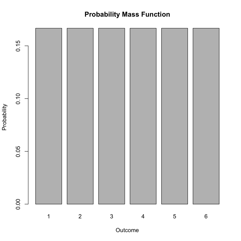
Consider the scenario of rolling a fair six-sided die. The outcome of this experiment follows a discrete uniform distribution, where each outcome has an equal probability of occurrence.

Table of Possible Values and Probabilities:

Outcome ( $x$ )	Probability ( $P (X = x)$ )
1	1/6
2	1/6
3	1/6
4	1/6
5	1/6
6	1/6

Visualization: The probability mass function (PMF) represents the probabilities associated with each possible outcome. In this case, it would be a histogram or bar plot where the height of each bar corresponds to the probability of the corresponding outcome.

The cumulative distribution function (CDF) shows the cumulative probability up to each possible outcome. It starts at zero and increases step by step as we move through the possible outcomes.

R Code:

# Define the outcomes and their corresponding probabilities
outcomes <- 1:6
probabilities <- rep(1/6, 6)

# Visualize PMF
barplot(probabilities, names.arg = outcomes, xlab = "Outcome", ylab = "Probability", main = "Probability Mass Function")

# Calculate CDF
cdf <- cumsum(probabilities)

# Visualize CDF
plot(outcomes, cdf, type = "s", xlab = "Outcome", ylab = "Cumulative Probability", main = "Cumulative Distribution Function")

_images/45a2c0c5c0503ba6f6828e769d08def0392bbbcec796d801c7125d2bd37ee7fd.png

_images/ce2a06c7264f31bb9738414bbfaf9d71f193ffac21ddb5874005c63d308948ac.png

Tip

In R’s plot() function, the type parameter specifies the type of plot to be drawn. Here are some common options:

"p": Points (scatter plot)
"l": Lines
"b": Both points and lines
"o": Overplotted points and lines
"h": Histogram-like vertical lines
"s": Stairs (step function)
"n": No plotting

For example, using type = "s" will create a step function plot.

The provided R code generates a plot representing the cumulative distribution function (CDF) for a discrete random variable. The plot consists of a step function where each step is represented by a horizontal line segment, extending from the left endpoint to the right endpoint of each step. Additionally, dots are placed at the left endpoints of the steps, and circles with holes are placed at the right endpoints. Furthermore, the plot extends the horizontal line segment from (6,1) to (7,1), representing the fact that the cumulative probability remains at 1 beyond the sixth outcome.

# Define the outcomes and their corresponding probabilities
outcomes <- 1:6
probabilities <- rep(1/6, 6)

# Calculate CDF
cdf <- cumsum(probabilities)

# Create an empty plot with specified x-axis and y-axis limits
plot(outcomes, type = "n", xlab = "Outcome", ylab = "Cumulative Probability", main = "Cumulative Distribution Function", xlim = c(0, 7), ylim = c(0, 1))

# Add the step function with segments of horizontal lines
for (i in 1:(length(outcomes)-1)) {
  segments(outcomes[i], cdf[i], outcomes[i+1], cdf[i], lwd = 2) # Horizontal lines
}

# Add dots at the left ends of each step
points(outcomes, cdf, pch = 19, cex = 1.5) # Dot (pch = 19)

# Add circles at the right ends of each step
for (i in 1:(length(outcomes)-1)) {
  points(outcomes[i+1], cdf[i], pch = 21, cex = 1.5) # Circle with hole (pch = 21)
}

# Draw a horizontal line extended from (6,1)
segments(6, 1, 7, 1, lwd = 2)

_images/6918ce6d854d424c96c9c754df57103b5eeacf76860a6e740be4b6fec183fd84.png

Poisson distribution#

Example 2.34: Discrete uniform distribution: Poisson Distribution for Number of Claims

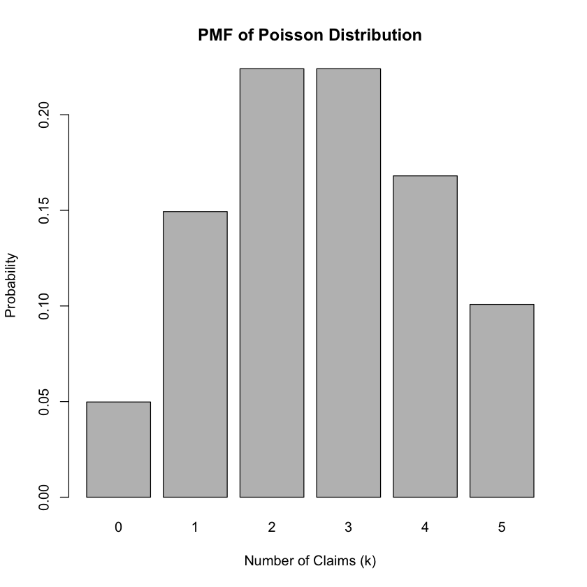
In insurance, the number of claims that arise up to a given time period can often be modeled using the Poisson distribution. This distribution is commonly used when dealing with count data, such as the number of accidents, claims, or arrivals in a fixed interval of time or space.

Probability Mass Function (PMF) and Cumulative Distribution Function (CDF)

The probability mass function (PMF) of the Poisson distribution is given by:

P (X = k) = \frac{e^{- λ} λ^{k}}{k!}

Where:

$X$ is the random variable representing the number of claims,
$k$ is a non-negative integer representing the number of claims,
$λ$ is the average rate of claims occurring per unit time.

The cumulative distribution function (CDF) of the Poisson distribution can be calculated as:

F (X \leq k) = \sum_{i = 0}^{k} \frac{e^{- λ} λ^{i}}{i!}

Example Table of Possible Values and Probabilities

Number of Claims ( $k$ )	Probability ( $P (X = k)$ )
0	$e^{- λ}$
1	$\frac{e^{- λ} λ}{1!}$
2	$\frac{e^{- λ} λ^{2}}{2!}$
…	…

Visualizing PMF and CDF

You can visualize the PMF by plotting the probabilities of different numbers of claims on a bar chart. For the CDF, you can plot the cumulative probabilities against the number of claims.

R Code Example

# Function to calculate PMF for Poisson distribution
pmf_poisson <- function(k, lambda) {
  return(exp(-lambda) * lambda^k / factorial(k))
}

# Function to calculate CDF for Poisson distribution
cdf_poisson <- function(k, lambda) {
  cdf <- rep(0, length(k))
  for (i in 1:length(k)) {
    cdf[i] <- sum(pmf_poisson(0:k[i], lambda))
  }
  return(cdf)
}

# Define parameters
lambda <- 3
k <- 0:5

# Calculate PMF
pmf_values <- pmf_poisson(k, lambda)
cat("PMF Values:", pmf_values, "\n")

# Calculate CDF
cdf_values <- cdf_poisson(k, lambda)
cat("CDF Values:", cdf_values, "\n")

# Plot PMF
barplot(pmf_values, names.arg = k, xlab = "Number of Claims (k)", ylab = "Probability", main = "PMF of Poisson Distribution")

# Plot CDF
plot(k, cdf_values, type = "s", xlab = "Number of Claims (k)", ylab = "Cumulative Probability", main = "CDF of Poisson Distribution")

PMF Values: 0.04978707 0.1493612 0.2240418 0.2240418 0.1680314 0.1008188

CDF Values: 0.04978707 0.1991483 0.4231901 0.6472319 0.8152632 0.9160821

_images/616b861bda468831a34f36c0f02db09834d6b1cc58a4ff2afd449de2da9e8c4c.png

_images/aa1b20e92ad834e69f5393d8cc07a80702f2c9ef2bf63af6b5315f971433c905.png

Binomial distribution#

Discrete Probability Distribution Example: Binomial Distribution in Actuarial Science

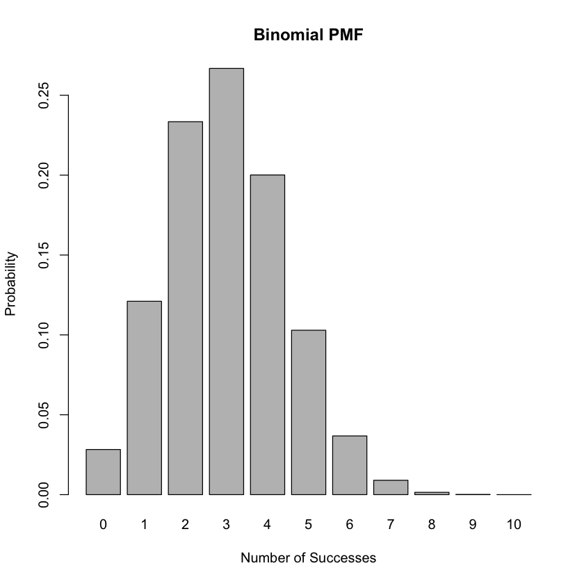
In actuarial science, the Binomial distribution is often used to model the number of successful outcomes in a fixed number of independent Bernoulli trials. It’s applicable in scenarios such as the number of travel insurance policies that result in at most one claim.

Probability Mass Function (PMF) and Cumulative Distribution Function (CDF)

The probability mass function (PMF) of the Binomial distribution is given by:

P (X = k) = (\binom{n}{k}) p^{k} (1 - p)^{n - k}

Where:

$X$ is the random variable representing the number of policies resulting in at most one claim,
$k$ is a non-negative integer representing the number of policies resulting in at most one claim,
$n$ is the total number of travel insurance policies,
$p$ is the probability that a policy results in at most one claim.

The cumulative distribution function (CDF) of the Binomial distribution can be calculated using the formula:

F (X \leq k) = \sum_{i = 0}^{k} (\binom{n}{i}) p^{i} (1 - p)^{n - i}

Example Table of Possible Values and Probabilities

Policies Resulting in at most One Claim ( $k$ )	Probability ( $P (X = k)$ )
0	$(1 - p)^{n}$
1	$(\binom{n}{1}) p (1 - p)^{n - 1}$
2	$(\binom{n}{2}) p^{2} (1 - p)^{n - 2}$
…	…

Visualizing PMF and CDF

You can visualize the PMF by plotting the probabilities of different numbers of policies resulting in at most one claim on a bar chart. For the CDF, you can plot the cumulative probabilities against the number of policies resulting in at most one claim.

R Code Example

# Example R code for Binomial distribution
n <- 10  # Number of trials
p <- 0.3  # Probability of success in each trial
k_values <- 0:n  # Number of successes
pmf <- dbinom(k_values, size = n, prob = p)  # Probability Mass Function
cdf <- pbinom(k_values, size = n, prob = p)  # Cumulative Distribution Function

# Plotting PMF
barplot(pmf, names.arg = k_values, xlab = "Number of Successes", ylab = "Probability", main = "Binomial PMF")

# Plotting CDF
plot(k_values, cdf, type = "s", xlab = "Number of Successes", ylab = "Cumulative Probability", main = "Binomial CDF")

_images/6c3b87fd09b057f5057f01bdd639e881ce541cbaa9792b834f90541fc8217df7.png

_images/3bf36a2771b7e7ab294edba208af8586df6eef94915f66c52959c9912623d4be.png

Expected Value and Variance of a Discrete Random Variable#

When dealing with random variables, understanding their expected value and variance is crucial for making predictions and analyzing outcomes. The expected value, denoted by $μ$ or $E (X)$ , represents the average value we anticipate from a random variable. Similarly, variance, denoted by $σ^{2}$ or $V a r (X)$ , measures how much the values of the random variable tend to deviate from the expected value.

Expected value

The expected value $μ$ or $E (X)$ of a discrete random variable $X$ with probability mass function $P (X)$ is calculated as:

μ = E (X) = \sum_{x} x \cdot P (X = x)

Variance

The variance $σ^{2}$ or $V a r (X)$ of the same random variable is given by:

σ^{2} = V a r (X) = \sum_{x} (x - μ)^{2} \cdot P (X = x)

Example 2.35: Calculation of expected value and variance

Consider the scenario of rolling a fair six-sided die. Let $X$ be the random variable representing the outcome of the roll.

The probability mass function for a fair six-sided die is $P (X = x) = \frac{1}{6}$ for $x = 1, 2, 3, 4, 5,$ and $6$ .

Expected Value:

μ = E (X) = \sum_{x = 1}^{6} x \cdot \frac{1}{6} = \frac{1}{6} (1 + 2 + 3 + 4 + 5 + 6) = \frac{21}{6} = 3.5

So, the expected value of rolling a fair six-sided die is $3.5$ .

Variance:

σ^{2} = V a r (X) = \sum_{x = 1}^{6} (x - 3.5)^{2} \cdot \frac{1}{6}

= \frac{1}{6} ((1 - 3.5)^{2} + (2 - 3.5)^{2} + (3 - 3.5)^{2} + (4 - 3.5)^{2} + (5 - 3.5)^{2} + (6 - 3.5)^{2})

= \frac{1}{6} (6.25 + 2.25 + 0.25 + 0.25 + 2.25 + 6.25)

= \frac{17.5}{6} = 2.916667

So, the variance of rolling a fair six-sided die is $2.916667$ .

Expected Value and Variance of a Continuous Random Variable#

Understanding the expected value and variance of continuous random variables is essential for analyzing processes where outcomes vary continuously, with the expected value representing the average outcome we anticipate, denoted by $μ$ or $E (X)$ , and variance indicating the degree of deviation from this expected value, denoted by $σ^{2}$ or $V a r (X)$ .

Formulas

The expected value $μ$ or $E (X)$ of a continuous random variable $X$ with probability density function $f (x)$ is calculated as:

μ = E (X) = \int_{- \infty}^{\infty} x \cdot f (x) d x

And the variance $σ^{2}$ or $V a r (X)$ of the same continuous random variable is given by:

σ^{2} = V a r (X) = \int_{- \infty}^{\infty} (x - μ)^{2} \cdot f (x) d x

Example 2.36: Calculation of expected value and variance

Consider the scenario where we model the time between insurance claims using the Exponential distribution. The Exponential distribution is commonly used to represent the waiting time until the occurrence of a continuous event. Let $X$ be the continuous random variable representing the time between claims.

For the Exponential distribution, the probability density function is given by:

f (x; λ) = λ e^{- λ x}

where $λ > 0$ is the rate parameter.

Suppose we have an insurance company with an average of 2 claims per day. We can model the time between claims with an Exponential distribution with $λ = 2$ .

Expected Value:

μ = E (X) = \int_{0}^{\infty} x \cdot λ e^{- λ x} d x

= \int_{0}^{\infty} x \cdot 2 e^{- 2 x} d x

= {[- x e^{- 2 x}]}_{0}^{\infty} + \int_{0}^{\infty} e^{- 2 x} d x

= {[- x e^{- 2 x} - \frac{1}{2} e^{- 2 x}]}_{0}^{\infty}

= 0 - (0 - \frac{1}{2}) = \frac{1}{2}

So, the expected value of the time between claims is $\frac{1}{2}$ days.

Variance:

σ^{2} = V a r (X) = \int_{0}^{\infty} (x - \frac{1}{2})^{2} \cdot 2 e^{- 2 x} d x

= {[- \frac{1}{4} (4 x^{2} + 1) e^{- 2 x}]}_{0}^{\infty}

= \frac{1}{4} .

So, the variance of the time between claims is $\frac{1}{4}$ days squared.

R Functions for Probability Distributions:#

In R, various functions are available for working with probability distributions.

For the Poisson distribution with parameter $λ$ , the density function $P (X = x)$ , distribution function $P (X \leq x)$ , quantile function (inverse cumulative distribution function), and random generation are provided as follows:

Poisson Distribution:

Poisson Distribution:
- Density function: dpois(x, lambda, log = FALSE): Computes the probability density function for the Poisson distribution at the specified values of $x$ with parameter $λ$ .
- Distribution function: ppois(q, lambda, lower.tail = TRUE, log.p = FALSE): Computes the cumulative distribution function for the Poisson distribution at the specified quantiles $q$ with parameter $λ$ .
- Quantile function (inverse c.d.f.): qpois(p, lambda, lower.tail = TRUE, log.p = FALSE): Computes the quantile function (inverse cumulative distribution function) for the Poisson distribution at the specified probabilities $p$ with parameter $λ$ .
- Random generation: rpois(n, lambda): Generates random deviates from the Poisson distribution with parameter $λ$ .

For the Binomial distribution with parameters $n$ and $p$ , similar functions are available:

Binomial Distribution:

Binomial Distribution:
- Density function: dbinom(x, size, prob, log = FALSE): Computes the probability mass function for the Binomial distribution at the specified values of $x$ with parameters $n$ (size) and $p$ (probability of success).
- Distribution function: pbinom(q, size, prob, lower.tail = TRUE, log.p = FALSE): Computes the cumulative distribution function for the Binomial distribution at the specified quantiles $q$ with parameters $n$ and $p$ .
- Quantile function (inverse c.d.f.): qbinom(p, size, prob, lower.tail = TRUE, log.p = FALSE): Computes the quantile function (inverse cumulative distribution function) for the Binomial distribution at the specified probabilities $p$ with parameters $n$ and $p$ .
- Random generation: rbinom(n, size, prob): Generates random deviates from the Binomial distribution with parameters $n$ and $p$ .

Similarly, for the Normal distribution:

Normal Distribution:

Normal Distribution:
- Density function: dnorm(x, mean = 0, sd = 1, log = FALSE): Computes the probability density function for the Normal distribution at the specified values of $x$ with parameters $μ$ (mean) and $σ$ (standard deviation).
- Distribution function: pnorm(q, mean = 0, sd = 1, lower.tail = TRUE, log.p = FALSE): Computes the cumulative distribution function for the Normal distribution at the specified quantiles $q$ with parameters $μ$ and $σ$ .
- Quantile function (inverse c.d.f.): qnorm(p, mean = 0, sd = 1, lower.tail = TRUE, log.p = FALSE): Computes the quantile function (inverse cumulative distribution function) for the Normal distribution at the specified probabilities $p$ with parameters $μ$ and $σ$ .
- Random generation: rnorm(n, mean = 0, sd = 1): Generates random deviates from the Normal distribution with parameters $μ$ and $σ$ .