2.2 Probability Basics#
Probability is essentially a way of quantifying uncertainty. In our daily lives, we are often faced with situations where we’re uncertain about the outcome. For example, when we flip a coin, we are uncertain whether it will land heads or tails. Probability helps us understand and measure that uncertainty.
In actuarial science, probability plays a crucial role in assessing risk and predicting future events, especially in insurance and finance. Actuaries use probability to analyze the likelihood of different outcomes, such as the probability of a person getting into a car accident or the probability of a house being damaged in a storm.
Definition
Probability is the measure of the likelihood that an event will occur.
Probability is typically represented as a number between 0 and 1, where 0 indicates that the event will not occur, and 1 indicates that the event will definitely occur. The closer the probability is to 1, the more likely the event is to occur, and the closer it is to 0, the less likely it is to occur.
Introduction to Events in Probability Theory#
In probability theory, an event is simply an outcome or a set of outcomes of an experiment or a random phenomenon. Events can range from simple outcomes, like flipping heads on a coin, to more complex outcomes involving multiple events, such as drawing a red card from a deck of playing cards.
Using R to simulate events#
Example 2.26 Rolling two six-sided dice
Explain what the sample space is for rolling two six-sided dice and provide examples of possible outcomes. Additionally, include R code to simulate this experiment.
Solution to Example 2.26
Sample Space: When rolling two six-sided dice, each die has six possible outcomes: 1, 2, 3, 4, 5, or 6. Therefore, the sample space consists of all possible combinations of outcomes from rolling two dice. Since each die roll is independent, there are \(6 \times 6 = 36\) possible outcomes in the sample space.
Events:
Event A: Event A represents the occurrence where the sum of the numbers rolled by two six-sided dice is 7.
Event B: Event B represents the occurrence where At least one die shows a 4.
Event C: Event C represents the occurrence where the two dice show the same number..
These examples illustrate different events that can occur when rolling two six-sided dice, each corresponding to specific outcomes within the sample space.
Here’s the R code to simulate the experiment of rolling two rolling of two six-sided dice and provides information on the outcomes and possible combinations.
# Simulate rolling two six-sided dice
die1 <- sample(1:6, 1, replace = TRUE)
die2 <- sample(1:6, 1, replace = TRUE)

# Display the outcomes and possible outcomes
cat("Outcomes of rolling two six-sided dice:")
cat("Die 1:", die1, "\n")
cat("Die 2:", die2, "\n")

# Display the possible outcomes for rolling two six-sided dice
cat("Possible outcomes for rolling two six-sided dice:\n")
outcomes <- expand.grid(1:6, 1:6)
for (i in 1:nrow(outcomes)) {
  cat("(", outcomes[i, 1], ", ", outcomes[i, 2], ")", sep = "")
  if (i < nrow(outcomes)) {
    cat(", ")
  }
}
Outcomes of rolling two six-sided dice:
Die 1: 1
Die 2: 2
Possible outcomes for rolling two six-sided dice:
(1, 1), (2, 1), (3, 1), (4, 1), (5, 1), (6, 1), (1, 2), (2, 2), (3, 2), (4, 2), (5, 2), (6, 2), (1, 3), (2, 3), (3, 3), (4, 3), (5, 3), (6, 3), (1, 4), (2, 4), (3, 4), (4, 4), (5, 4), (6, 4), (1, 5), (2, 5), (3, 5), (4, 5), (5, 5), (6, 5), (1, 6), (2, 6), (3, 6), (4, 6), (5, 6), (6, 6)
This R code simulates the rolling of two six-sided dice and provides information on the outcomes and possible combinations.
Initially, it randomly generates the outcomes for each die roll using the
sample()function, storing the results in variablesdie1anddie2. Subsequently, the code displays the outcomes of each die roll.Additionally, it calculates and displays all possible outcomes for rolling two six-sided dice in tuple format
(x, y), wherexandyrepresent the numbers rolled on each die. This is achieved by creating all possible combinations of rolls using theexpand.grid()function and then iterating through each combination to display it accordingly.
Example 2.27 Simulation of Fire Damage in Insured Homes
The experiment in Example 2.23 aims to assess fire damage in 1000 insured homes by simulation using R.
To simulate the event of an insurance company offering a policy that covers damages to homes due to fire in R, you can follow these steps:
Define the parameters of your simulation, such as the number of policies sold and the probability of a house experiencing fire damage.
Simulate whether each house covered by the policy experiences fire damage or not using random number generation.
Repeat the simulation process multiple times to generate a distribution of outcomes.
Here’s an example code in R:
# Set the parameters
num_policies <- 1000  # Number of policies sold
fire_prob <- 0.05     # Probability of a house experiencing fire damage

# Simulate the event for each policy
fire_damage <- rbinom(num_policies, 1, fire_prob)

# Count the number of houses with fire damage
num_houses_damaged <- sum(fire_damage)

# Calculate the proportion of houses with fire damage
proportion_damaged <- num_houses_damaged / num_policies

# Print the results
cat("Number of houses with fire damage:", num_houses_damaged, "\n")
cat("Proportion of houses with fire damage:", proportion_damaged, "\n")
Number of houses with fire damage: 48
Proportion of houses with fire damage: 0.048
In this example, we use the rbinom() function to simulate whether each house covered by the policy experiences fire damage or not.
Syntax and Arguments for rbinom()
rbinom(n, size, prob)
n: Represents the number of observations you want to simulate.size: Specifies the number of trials per observation.prob: Indicates the probability of success for each trial.
The rbinom() function generates random binomial variates, where we set size to 1 because each policy is treated as an independent observation, and we’re interested in a single trial (observation) for each policy. The resulting vector of random numbers fire_damage consists of 1s, representing fire damage, and 0s, indicating no damage, based on the specified probability fire_prob. We repeat this process num_policies times to simulate the event for each policy.
You can adjust the parameters num_policies and fire_prob to reflect different scenarios and run the simulation multiple times to observe variations in outcomes.
The Binomial and Bernoulli distributions
The Binomial distribution and the Bernoulli distribution are closely related concepts in probability theory, often used to model the number of successes in a fixed number of independent Bernoulli trials.
Bernoulli Distribution: This distribution represents the outcome of a single Bernoulli trial, which is a random experiment with only two possible outcomes: success (usually denoted as 1) and failure (usually denoted as 0). The Bernoulli distribution is characterized by a single parameter, usually denoted as p, which represents the probability of success. The probability mass function (PMF) of the Bernoulli distribution is given by:
where \(X\) is the random variable representing the outcome of the Bernoulli trial.
Binomial Distribution: The Binomial distribution extends the concept of the Bernoulli distribution to describe the number of successes (or failures) in a fixed number of independent Bernoulli trials. It is characterized by two parameters: \(n\), the number of trials, and \(p\), the probability of success in each trial. The probability mass function (PMF) of the Binomial distribution is given by:
where \(X\) is the random variable representing the number of successes, \(k\) is the number of successes (which can range from 0 to \(n\)), \(n\) is the total number of trials, and \(p\) is the probability of success in each trial.
Probability of an event#
Probability is a fundamental concept in mathematics and statistics that quantifies the likelihood of an event occurring. Whether it’s predicting the outcome of a dice roll, the chances of rain tomorrow, or the risk of an insurance claim, probability provides a framework for understanding uncertainty and making informed decisions in various fields.
Calculating Probability#
When all outcomes are equally likely, the probability of an event, denoted as \(P(A)\), is calculated by dividing the number of favorable outcomes by the total number of possible outcomes. This can be expressed as:
Consider a standard six-sided die. To calculate the probability of rolling a 3, there is only one favorable outcome (rolling a 3) out of six possible outcomes (rolling any number from 1 to 6). Therefore, the probability of rolling a 3 is \(\frac{1}{6}\).
Applications in Actuarial Science#
Actuarial science utilizes probability theory extensively to assess risk and uncertainty in insurance and finance. For example, actuaries use probability to determine insurance premiums by estimating the likelihood of policyholders making claims.
Let’s say an insurance company wants to calculate the probability of a 40-year-old male policyholder experiencing a heart attack within the next year. Actuaries collect data on similar individuals and analyze factors such as age, health history, lifestyle, and medical conditions. Based on historical data and statistical models, they estimate the probability of a heart attack occurring within a specific time frame for this demographic.
Actuaries also use probability to model financial risks, such as fluctuations in investment returns or the likelihood of loan defaults. By understanding the probabilities associated with different scenarios, they can help businesses and organizations make informed decisions to manage and mitigate risks effectively.
In actuarial science, precise probability calculations and accurate risk assessments are essential for maintaining the financial stability of insurance companies, pension funds, and other financial institutions.
Introduction to Empirical Probability#
Empirical probability, also known as experimental probability, is a method of determining the likelihood of an event based on observations or experiments. Unlike theoretical probability, which relies on mathematical calculations and assumptions about the underlying probabilities of events, empirical probability is derived from actual data obtained through observation or experimentation.
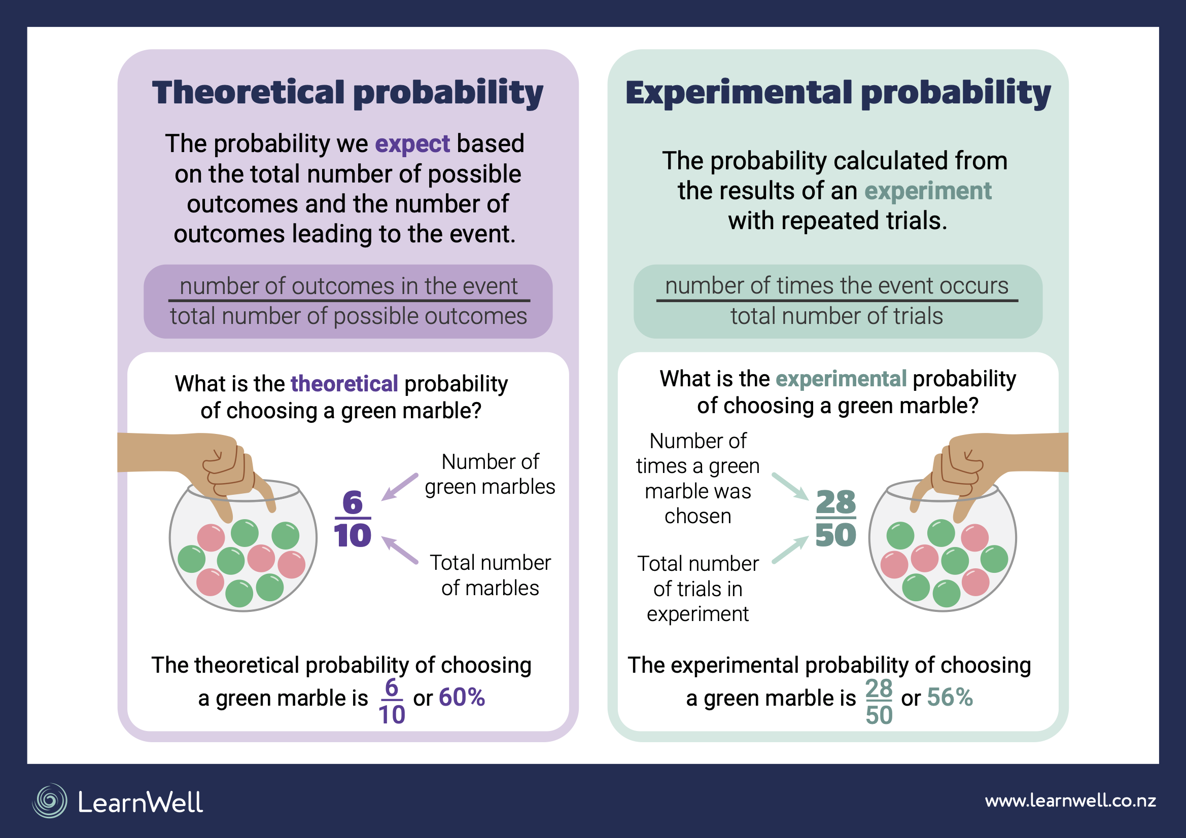
Fig. 8 Theoretical: based on mathematical principles and Empirical: based on observed data.#
Calculating Empirical Probability#
To calculate empirical probability, you simply count the number of times the event of interest occurs and divide it by the total number of trials or observations. This can be expressed as:
Let’s consider a simple example to illustrate empirical probability:
Example 2.28 Coin Toss
Suppose you want to determine the probability of landing heads when flipping a coin. You conduct an experiment where you flip the coin 100 times and record the outcomes. After completing the experiment, you find that the coin lands heads 47 times.
To calculate the empirical probability of landing heads:
So, based on your experiment, the empirical probability of landing heads when flipping this particular coin is 0.47 or 47%.
Importance of Empirical Probability#
Empirical probability is valuable because it provides real-world insights into the likelihood of events based on observed data. It is particularly useful when theoretical probabilities are difficult to determine or when there is limited information about the underlying probabilities.
By conducting experiments and collecting data, we can estimate probabilities for various events and make informed decisions in areas such as science, business, sports, and gambling. However, it’s important to note that empirical probabilities may vary depending on the sample size and the conditions of the experiment, so larger sample sizes generally lead to more reliable estimates.
Example 2.29
Write R code to simulate flipping a coin and use the simulation results to calculate the empirical probability of landing heads.
Simulate flipping a fair coin 100 times and record the outcomes. Then, calculate the empirical probability of landing heads based on the simulation results.
Relationship between Empirical and Theoretical Probabilities#
Empirical and theoretical probabilities are related in that they both aim to quantify the likelihood of events occurring.
Empirical probabilities can be used to validate theoretical predictions. For example, if theoretical calculations suggest that a coin should land heads 50% of the time, conducting a large number of coin flips and observing the frequency of heads can verify whether this theoretical prediction holds true in practice.
In situations where empirical data is unavailable or impractical to obtain, theoretical probabilities serve as a basis for making predictions and decisions.
Additionally, theoretical probabilities can be used to guide the design of experiments to collect empirical data. For instance, theoretical calculations may help determine the sample size needed for an experiment to achieve a desired level of confidence in the empirical results.
In summary, while empirical and theoretical probabilities differ in their methods of calculation and underlying assumptions, they are complementary approaches that contribute to our understanding and prediction of uncertain events.
Law of large numbers#
The relationship between empirical and theoretical probabilities is made evident by the Law of Large Numbers, which suggests that as the number of trials in an experiment increases, the observed empirical probability tends to converge towards the theoretical probability.
Illustrative Examples Demonstrating the Connection between Empirical and Theoretical Probabilities#
Coin Toss Experiment: Imagine flipping a fair coin repeatedly. Initially, the empirical probability of landing heads may fluctuate, but as the number of flips increases, it tends to stabilize around the theoretical probability of 0.5. This convergence demonstrates the Law of Large Numbers in action, as the observed empirical probability aligns more closely with the theoretical probability with a larger number of trials.
Dice Rolling Experiment: Similarly, consider rolling a fair six-sided die multiple times. Initially, the empirical probability of rolling a specific number may vary, but with more rolls, it tends to approach the theoretical probability of 1/6 for each face of the die. Again, this exemplifies how the Law of Large Numbers manifests the convergence of empirical probabilities towards theoretical expectations with increased trials.
Law of Large Numbers
The Law of Large Numbers states that as the number of repetitions in an experiment increases, the ratio of successful outcomes to the total number of trials tends to converge towards the theoretical probability of a single trial’s outcome.
Exploring the Relationship between Empirical and Theoretical Probabilities#
In this example, we will demonstrate how the empirical probabilities of rolling a fair six-sided die converge to the theoretical probabilities as the number of trials increases.
# Set the number of trials
num_trials <- 1000

# Roll a fair six-sided die 'num_trials' times
die_rolls <- sample(1:6, num_trials, replace = TRUE)

# Calculate empirical probabilities
empirical_prob <- table(die_rolls) / num_trials

# Theoretical probabilities for a fair six-sided die
theoretical_prob <- rep(1/6, 6)

# Output empirical and theoretical probabilities
print("Empirical Probabilities:")
print(empirical_prob)
print("Theoretical Probabilities:")
print(theoretical_prob)
[1] "Empirical Probabilities:"
die_rolls
    1     2     3     4     5     6
0.160 0.162 0.164 0.165 0.179 0.170
[1] "Theoretical Probabilities:"
[1] 0.1666667 0.1666667 0.1666667 0.1666667 0.1666667 0.1666667
Result Explanation
When you run the provided R code, it simulates rolling a fair six-sided die a specified number of times (num_trials). The empirical probabilities are calculated by dividing the frequency of each outcome by the total number of trials. The theoretical probabilities for a fair six-sided die are simply 1/6 for each outcome.
As you increase the number of trials (num_trials), you will notice that the empirical probabilities start to converge towards the theoretical probabilities. This convergence demonstrates the Law of Large Numbers, which states that as the number of trials increases, the empirical probabilities approach the theoretical probabilities. Thus, this example illustrates the connection between empirical and theoretical probabilities through the experiment of rolling a fair six-sided die multiple times.
Convergence of Empirical Probabilities with Increasing Trials#
In this subsection, we will investigate how the empirical probabilities of rolling a fair six-sided die converge to the theoretical probabilities as the number of trials increases. We will vary the number of trials from 100 to 1000 in increments of 100 and observe the behavior of the empirical probabilities.
Example 2.30
Can you use R to explore how the empirical probabilities of rolling a fair six-sided die approach the theoretical probabilities as you increase the number of trials from 100 to 1000 in increments of 100? Plot the number of trials against the empirical probabilities for each outcome and observe how they converge towards the theoretical probabilities.
# Initialize vector to store empirical probabilities
empirical_probs <- matrix(NA, nrow = 6, ncol = 10)

# Vary the number of trials from 100 to 1000 in increments of 100
for (i in 1:10) {
  num_trials <- i * 100

  # Roll a fair six-sided die 'num_trials' times
  die_rolls <- sample(1:6, num_trials, replace = TRUE)

  # Calculate empirical probabilities
  empirical_prob <- table(die_rolls) / num_trials

  # Store empirical probabilities
  empirical_probs[, i] <- empirical_prob
}

# Plot num_trials vs empirical probabilities for each outcome
plot(seq(100, 1000, by = 100), empirical_probs[1, ], type = "b",
     xlab = "Number of Trials", ylab = "Empirical Probability",
     main = "Convergence of Empirical Probabilities (Outcome: 1)")
for (i in 2:6) {
  points(seq(100, 1000, by = 100), empirical_probs[i, ], type = "b", col = i)
}
legend("topright", legend = c("Outcome 1", "Outcome 2", "Outcome 3", "Outcome 4", "Outcome 5", "Outcome 6"),
       col = 1:6, pch = 1, bty = "n")
Result Explanation
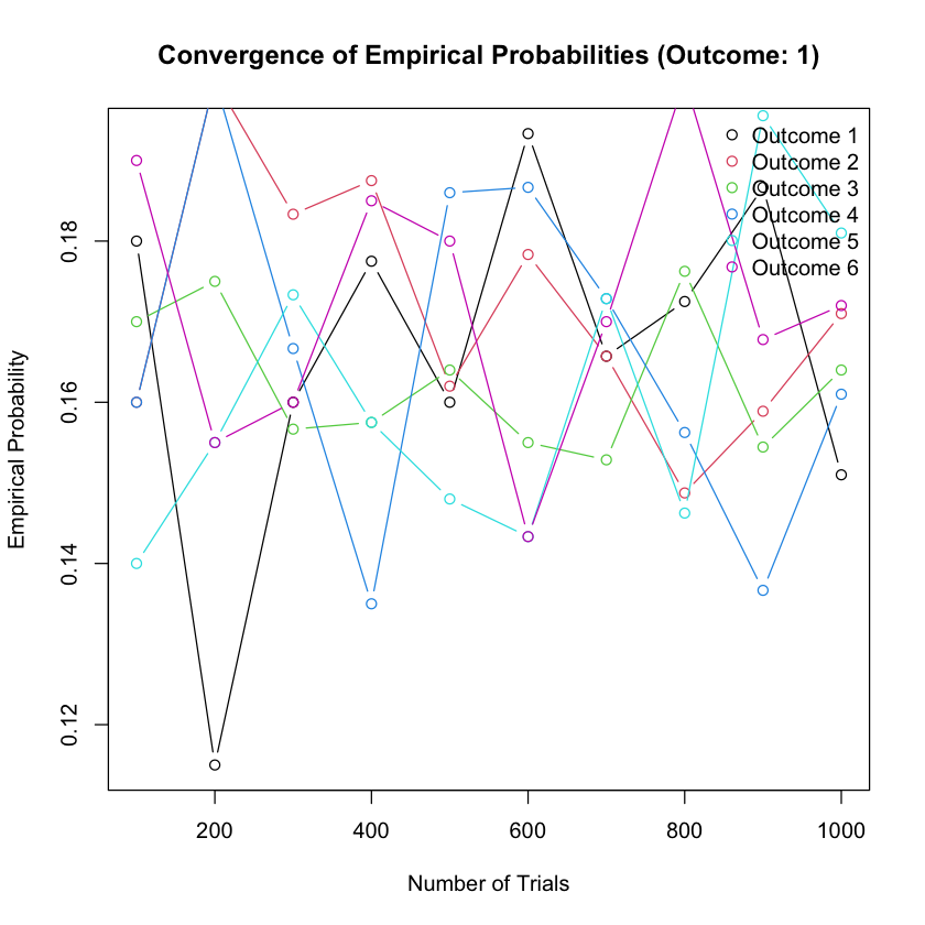
The provided R code calculates empirical probabilities for rolling a fair six-sided die with varying numbers of trials from 100 to 1000 in increments of 100. It then plots the number of trials against the empirical probabilities for each outcome.
As you observe the plot, you’ll notice that as the number of trials increases, the empirical probabilities for each outcome converge towards the theoretical probability of 1/6. This convergence is indicative of the Law of Large Numbers, demonstrating that with more trials, the empirical probabilities tend to approach the theoretical probabilities. Each line represents the convergence of empirical probabilities for a specific outcome as the number of trials increases.
Probability Properties#
In this section, we explore fundamental properties of probability that underpin its interpretation and application in various contexts.
Probability of an Event#
Probabilities are constrained within the range of 0 to 1, inclusively. A probability of 0 indicates that the event is impossible, while a probability of 1 signifies certainty that the event will occur. Intermediate probabilities closer to 0 suggest the event is less likely, whereas values nearing 1 indicate a high likelihood of occurrence. The probability of an event \(A\) is denoted as \(P(A)\).
Range of Probability for Any Event \(A\)#
The probability of any event \(A\) always falls within the inclusive range of 0 to 1.
Probability of a Complement#
The complement of an event \(A\), denoted as \(A'\), represents all outcomes not included in event \(A\). The probability of the complement of \(A\), denoted as \(P(A')\), is equal to 1 minus the probability of \(A\).
Probability of the Empty Set#
The empty set, denoted as \(\emptyset\), represents an event that cannot occur. Therefore, the probability of the empty set is 0.
If \(A\) and \(B\) are mutually exclusive, then \(P(A \cap B) = \emptyset\). Therefore,
Probability of the Union of Two Events#
The probability of the union of two events \(A\) and \(B\), denoted as \(P(A \cup B)\), represents the likelihood of either event \(A\) or event \(B\), or both, occurring.
For general events A and B, the probability of their union is given by:
If A and B are mutually exclusive, then