2.1 Data Collection and Descriptive Statistics#
In actuarial science, the foundational processes of data collection and descriptive statistics play a pivotal role in understanding and quantifying risk. Accurate and comprehensive data serves as the foundation for reliable information for actuarial analyses,collection providing essential insights into the patterns and characteristics of events under consideration.
Descriptive statistics, in turn, facilitate the concise summarization and interpretation of this data, serving as a crucial step in the actuarial decision-making process by enabling professionals to derive meaningful conclusions and assess potential financial implications.
Basic terms in statistics are illustrated in the following example.
Example 2.3
An actuarial student is interested in exploring the average income of policyholders in an actuarial portfolio. Applying the concepts in the context of actuarial science:
Population: The entire collection of incomes earned by all policyholders in the actuarial portfolio.
Sample: A subset of the population, such as the incomes of policyholders within a specific demographic or policy category.
Variable: The “income” assigned to each individual policyholder.
Data Value: For instance, the income of a specific policyholder, like Ms. Johnson’s income at $60,000.
Data: The set of values corresponding to the obtained sample (e.g., $60,000; $45,000; $75,000; …).
Experiment: The methods employed to select policyholders for the sample and determine the income of each, which could involve analyzing demographic data or using actuarial models.
Parameter: The sought-after information concerns the “average” income of all policyholders in the entire portfolio.
Statistic: The determined “average” income of policyholders within the selected sample.
Exploring Actuarial Data Collection#
In the field of actuarial science, various methods are commonly employed for data collection:
Actuarial Interviews Individuals often provide responses when interviewed by an actuarial professional, but their answers may be influenced by the interviewer’s approach, for e.g., an actuarial interview aiming to assess individuals’ perception of insurance risk.
Phone Surveys A cost-effective method, but it is essential to keep surveys brief as respondents in actuarial contexts may have limited patience.
Self-Administered Actuarial Questionnaires An economical option, yet the response rate may be lower, and the participants might constitute a biased sample in actuarial analyses.
Direct Risk Observation For specific risk factors, an actuary may directly observe and measure quantities of interest within the sample.
Web-Based Risk Surveys This method is limited to the population using the web, catering to a specific subset of individuals in actuarial investigations.
Tip
it is imperative to employ sampling methods for data collection that ensure the obtained data accurately represents the population and is free from bias.
Strategies for Collecting Data#
Data collection is a crucial step in the research process, and the selection of observations or measurements for a study depends on the research question and the goals of the study. There are two broad categories of methods for collecting data: non-probability methods and probability methods.
Non-Probability Methods#
Convenience or Haphazard Sampling: In convenience or haphazard sampling, units are chosen without a planned method, assuming population homogeneity. For instance, a vox pop survey randomly selects individuals passing by, introducing biases based on the interviewer’s decisions and the characteristics of those present during sampling.
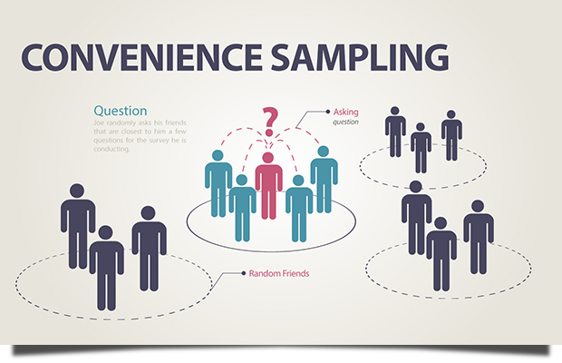
Fig. 4 Convenience Sampling#
Example 2.4
Imagine estimating life expectancy by randomly selecting individuals waiting in line at an insurance office for an actuarial study; however, this may introduce biases if those in line have specific characteristics.
Volunteer Sampling: Volunteer sampling involves including only willing participants, often with specific criteria. For example, in a radio show discussion, only those with strong opinions may respond, causing a selection bias as the silent majority typically does not participate.
Example 2.5
Understanding financial behaviors within an insurance portfolio may involve volunteer sampling by inviting policyholders to participate; however, biases may occur if those who volunteer have unique characteristics not representative of the entire group.
Probability Methods#
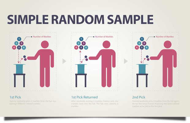
Simple Random Sample: Simple random sampling involves selecting units from a population in a completely random manner, ensuring every unit has an equal chance of being chosen. For example, drawing names from a hat for a survey is a simple random sampling method, minimizing biases and providing a representative sample.

Fig. 5 Simple Random Sampling#
Example 2.6
Estimating the average lifespan of policyholders by randomly selecting a subset for study through the use of randomly generated numbers is an application of simple random sampling, ensuring unbiased representation.
Stratified Random Sampling: Stratified random sampling involves dividing the population into subgroups (strata) based on certain characteristics and then randomly selecting samples from each stratum. For instance, when studying a diverse population, dividing it into age groups and then randomly selecting individuals from each group ensures representation across different age ranges, providing more accurate insights.
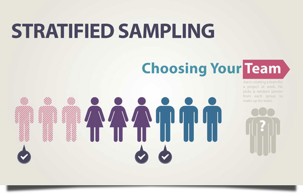
Fig. 6 Stratified Sampling#
Example 2.7
Estimating insurance claims across various demographic groups could involve stratified random sampling by categorizing policyholders based on income levels and then selecting samples from each stratum, ensuring a more subtle understanding of claim patterns.
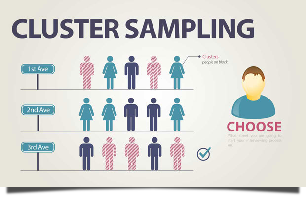
Cluster Sampling: Cluster sampling involves dividing the population into clusters and randomly selecting entire clusters for inclusion in the sample. For example, when studying a large geographical area, dividing it into clusters (such as cities or neighborhoods) and randomly selecting some clusters for analysis can be more practical than trying to include every individual unit, saving time and resources.

Fig. 7 Cluster Sampling#
Example 2.8
Assessing the risk profile of policyholders in various regions might involve cluster sampling by randomly selecting specific cities or towns as clusters and then studying all policyholders within those selected areas, providing insights into regional risk patterns.
Considerations in Data Collection#
Sampling Frame:
The list or source from which the sample is drawn.
Should represent the entire population.
Sample Size:
Balancing precision with practical considerations.
Larger samples increase representativeness but may be impractical.
Data Collection Tools:
Choosing appropriate instruments for measurement (surveys, interviews, etc.).
Depends on research objectives.
Ethical Considerations:
Ensuring participant rights through informed consent and confidentiality.
Adherence to ethical guidelines.
In conclusion, the choice between non-probability and probability methods depends on the research design, resources, and the level of representativeness required. Both methods have their strengths and limitations, and researchers must carefully consider these factors when selecting their data collection approach.
Sampling Methods in R#
This section explores various techniques for obtaining subsets of data from larger datasets using the R programming language. Understanding and implementing these sampling methods is fundamental to achieving accurate and reliable insights from data, contributing to the robustness of statistical analyses and research findings.
Simple Random Sampling in R#
To obtain a random sample, one can sequentially label all cases and generate uniformly distributed random numbers for selecting cases from the population.
In R, a simple random sample can be generated using the sample() function. The function is defined as follows:
sample(x, size, replace = FALSE, prob = NULL)
Example 2.9
How can the acceptability of a sample, drawn through simple random sampling from a normal distribution with a given mean (\(\mu\)) and standard deviation (\(\sigma\)), be evaluated? The evaluation includes comparing histograms and conducting basic statistical checks to ensure the sample adequately represents the population.
Objective: Evaluate the acceptability of a sample drawn through simple random sampling from a normal distribution.
Tasks:
Generate a large population (\(N\)) following a normal distribution with a specified mean (\(\mu\)) and standard deviation (\(\sigma\)).
Draw a sample (\(n\)) from the population using simple random sampling.
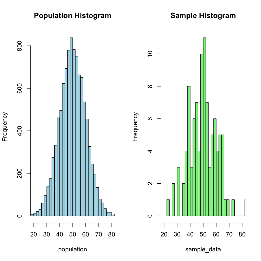
Compare the histograms of the population and the sample to visually inspect their distributions.
Perform basic statistical checks, including calculating means and variances, to assess the representativeness of the sample.
Optionally, conduct a t-test to further validate the similarity between the sample and the population.
# Set seed for reproducibility
set.seed(123)

# Parameters
N <- 10000        # Population size
mu <- 50          # Mean of the population
sigma <- 10       # Standard deviation of the population
n <- 100          # Sample size

# Step 1: Create a population following a normal distribution
population <- rnorm(N, mean = mu, sd = sigma)

# Step 2: Draw a sample using simple random sampling
sample_data <- sample(population, size = n)

# Step 3: Compare the histogram of the population and the sample
par(mfrow = c(1, 2))

hist(population, main = "Population Histogram", col = "lightblue", xlim = c(20, 80), breaks = 30)
hist(sample_data, main = "Sample Histogram", col = "lightgreen", xlim = c(20, 80), breaks = 30)

# Step 4: Verify that the sample is acceptable
# You can perform statistical tests or compare summary statistics

# For example, compare means and variances
cat("Population Mean:", mean(population), "\n")
cat("Sample Mean:", mean(sample_data), "\n")

cat("Population Variance:", var(population), "\n")
cat("Sample Variance:", var(sample_data), "\n")

# Alternatively, you can perform a t-test if the population parameters are known
t_test_result <- t.test(sample_data, mu = mu)
cat("\nT-test p-value:", t_test_result$p.value, "\n")

# You can also visually inspect the histograms and summary statistics to check for bias

# Reset the par settings
par(mfrow = c(1, 1))
Population Mean: 49.97628
Sample Mean: 49.93819
Population Variance: 99.72751
Sample Variance: 115.2845
T-test p-value: 0.9542086
Tip
Null Hypothesis for T-Test:
\( H_0: \mu_{\text{sample}} = \mu_{\text{population}} \)
Where:
\( \mu_{\text{sample}} \) is the mean of the sample.
\( \mu_{\text{population}} \) is the known or hypothesized mean of the population.
The null hypothesis posits that there is no significant difference between the mean of the sample and the specified mean of the population. The t-test will assess whether any observed differences are statistically significant or if they could likely occur due to random sampling variability.
Conclusion from T-Test:
With a p-value of 0.9542086 obtained from the t-test, we fail to reject the null hypothesis (\( H_0: \mu_{\text{sample}} = \mu_{\text{population}} \)). This suggests that there is not enough statistical evidence to conclude that the mean of the sample is significantly different from the specified mean of the population. The observed differences are likely attributable to random sampling variability.
Stratified Sampling in R#
In stratified sampling, the population is divided into smaller subgroups, or strata, based on common factors such as age, gender, income, etc. These strata are designed to accurately represent the overall population.
For instance, when examining the daily time spent on messaging for male and female users, the strata may be defined as male and female users, and random sampling is then applied within each gender stratum.
Tip
It’s important to note that while stratified sampling provides more precise estimates compared to random sampling, a major drawback is the need for knowledge about the specific characteristics of the population, which may not always be readily available. Additionally, determining the appropriate characteristics for stratification can pose challenges.
Balanced and Imbalanced Dataset#
In the following examples, we will create two different synthetic datasets and implement stratified sampling, a technique crucial for maintaining proportional representation within distinct subgroups or strata.
The initial dataset, representing a balanced distribution, guarantees that each category is evenly presented within its own subgroup. This creates an inclusive learning environment where all classes have a fair presence.
Conversely, the second dataset deliberately introduces an imbalance. Here, certain classes are intentionally presented in smaller numbers within their respective subgroups. This intentional imbalance reflects real-world situations where certain scenarios require focused attention on specific classes.
Stratified sampling becomes essential in preserving proportional class representation within each subgroup, a methodology particularly valuable in both balanced and imbalanced cases.
Balanced Dataset: A balanced dataset is characterized by an equal or nearly equal distribution of instances across different classes or categories. In other words, each class in the dataset has a comparable number of samples.
Imbalanced Dataset: An imbalanced dataset occurs when the number of instances in different classes significantly varies. One or more classes might be underrepresented, making it challenging for a model to learn patterns associated with the minority class(es).
Example 2.10 Synthetic balanced datasets
We aim to perform stratified sampling on a synthetic balanced dataset using the dplyr package in R. The dataset contains two classes, “ClassA” and “ClassB,” and we intend to create a representative sample while maintaining the balance between the classes. The following tasks will be executed:
Tasks for Stratified Sampling on Synthetic Imbalanced Datasets:
Install and Load Packages:
Use
install.packagesto install the necessary packages.Load the
dplyrlibrary for data manipulation.
Create a Balanced Dataset:
Generate a synthetic dataset with two features, “feature1” and “feature2,” and 200 observations.
The dataset is balanced, with 100 instances for each class.
Stratified Sampling:
Utilize the
group_byandsample_nfunctions fromdplyrto perform stratified sampling.Ensure that the sample size is set to 50 for each class to maintain balance.
Display the Result:
Use the
tableorprop.tablefunction to present the counts or proportions of each class within the sampled data subgroups.This will provide insights into the distribution of classes within the stratified sample, considering the intentional imbalance in the dataset.
# Load the dplyr package
suppressMessages(library(dplyr))

# Create a balanced dataset
set.seed(123)
data_balanced <- data.frame(
  feature1 = rnorm(200, mean = 5),
  feature2 = rnorm(200, mean = 10),
  class = rep(c("ClassA", "ClassB"), each = 100)
)

# Stratified sampling for a balanced dataset
sampled_data_balanced <- data_balanced %>%
  group_by(class) %>%
  sample_n(size = 50) %>%
  ungroup()

# Display the result
prop.table(table(sampled_data_balanced$class))
ClassA ClassB
   0.5    0.5
Tip
In the obtained result for the balanced case, the stratified sampling successfully yielded a distribution of classes where both ‘ClassA’ and ‘ClassB’ are evenly represented, each constituting 50% of the stratified sample.
Example 2.11 Synthetic imbalanced datasets
We aim to perform stratified sampling on a synthetic imbalanced dataset using the dplyr package in R. The dataset comprises two classes, “ClassA” and “ClassB,” intentionally structured to demonstrate imbalance. The objective is to create a representative sample while acknowledging and addressing the intentional underrepresentation of specific classes within their respective subgroups.
Tasks for Stratified Sampling on Synthetic Imbalanced Datasets
Install and Load Packages:
Use
install.packagesto install the necessary packages.Load the
dplyrlibrary for data manipulation.
Create an Imbalanced Dataset:
Generate a synthetic dataset with two features, “feature1” and “feature2,” and 200 observations.
Intentionally structure the dataset to illustrate imbalance, with specific classes deliberately underrepresented within their corresponding subgroups.
Stratified Sampling for Imbalanced Dataset:
Utilize the
group_byandsample_fracfunctions fromdplyrto perform stratified sampling.Set the
sizeparameter to sample a fraction (e.g., 0.5) of the observations from each class, allowing for replacement (replace = TRUE) to address intentional underrepresentation.
Display the Result:
Use the
tableorprop.tablefunction to present the counts or proportions of each class within the sampled data subgroups.This will provide insights into the distribution of classes within the stratified sample, considering the intentional imbalance in the dataset.
Adjust parameters and explore various sampling strategies based on the specific requirements of your imbalanced dataset.
# Create an imbalanced dataset
set.seed(123)
data_imbalanced <- data.frame(
  feature1 = rnorm(200, mean = 5),
  feature2 = rnorm(200, mean = 10),
  class = c(rep("ClassA", 180), rep("ClassB", 20))
)

# Stratified sampling for an imbalanced dataset using sample_frac
sampled_data_imbalanced <- data_imbalanced %>%
  group_by(class) %>%
  sample_frac(size = 0.5, replace = TRUE) %>%
  ungroup()

# Display the result
prop.table(table(sampled_data_imbalanced$class))
ClassA ClassB
   0.9    0.1
In this example, sample_frac is used to sample 50% of the observations from each group (size = 0.5). The replace = TRUE argument allows for replacement, which is necessary when sampling a fraction that exceeds the number of available observations in the minority class.
Using sample_frac helps maintain the relative imbalance in the dataset while ensuring that the sampled dataset has a representative mix of both majority and minority classes. Adjust the size parameter according to your specific sampling requirements.
Case Study: mtcars Dataset#
You can use other datasets related to business, economics, or finance to apply the same stratified sampling code in R. One such dataset is the “mtcars” dataset, which is included in the base R package. It contains information about various car models, including attributes such as miles per gallon (mpg), number of cylinders, and horsepower. You can stratify the sampling based on the number of cylinders in this dataset.
Example 2.12 mtcars dataset
In the analysis of the mtcars dataset, we aim to explore and understand the characteristics of different subgroups based on the number of cylinders in each vehicle. To facilitate this investigation, a new categorical variable named “CylinderGroup” has been introduced, utilizing the ‘cut’ function to stratify the data into three distinct groups: “Low,” “Medium,” and “High,” representing vehicles with 3-4 cylinders, 5-6 cylinders, and 7-8 cylinders, respectively. This stratification allows us to create meaningful subgroups for further analysis. As part of our analytical approach, we will employ stratified sampling techniques to ensure that our sample accurately reflects the proportion of vehicles in each cylinder group. This approach enables us to draw meaningful insights by considering the unique characteristics and variations within each cylinder subgroup, contributing to a more nuanced understanding of the mtcars dataset.
Descriptive Statistics#
Descriptive statistics is a branch of statistics that involves the collection, analysis, interpretation, presentation, and organization of data. In general, data can be classified into two main types: Qualitative (Categorical) and Quantitative.
Types of Data#
Qualitative (Categorical)#
Qualitative data represents categories and can be divided into three subtypes:
Binary
Data with only two possible values, making it a binary choice. In actuarial science, examples include:
Gender (Male/Female)
Policy Status (Active/Inactive)
Ordinal
Data with ordered categories that hold a meaningful sequence. Actuarial examples encompass:
Policy Rating (Low/Medium/High)
Customer Satisfaction Level (Low/Medium/High)
Nominal
Data with categories that lack a specific order. Actuarial instances comprise:
Marital Status (Single/Married/Divorced)
Type of Insurance (Life/Health/Property)
Quantitative#
Quantitative data involves numerical values and is further categorized into two types:
Discrete
Data with distinct, separate values. In actuarial science, examples include:
Number of Policies Sold
Count of Claims in a Year
Continuous
Data that can take any value within a given range. Actuarial examples comprise:
Policy Premium Amount
Policyholder Age
Data Type Exploration in R#
You can use various functions to identify the types of data in a dataset. The str() function is particularly useful for this purpose. For the mtcars dataset, you can use the following code to display information about the types of data:
# Load the mtcars dataset
data(mtcars)

# Display the structure of the dataset
str(mtcars)
'data.frame':	32 obs. of  11 variables:
 $ mpg : num  21 21 22.8 21.4 18.7 18.1 14.3 24.4 22.8 19.2 ...
 $ cyl : num  6 6 4 6 8 6 8 4 4 6 ...
 $ disp: num  160 160 108 258 360 ...
 $ hp  : num  110 110 93 110 175 105 245 62 95 123 ...
 $ drat: num  3.9 3.9 3.85 3.08 3.15 2.76 3.21 3.69 3.92 3.92 ...
 $ wt  : num  2.62 2.88 2.32 3.21 3.44 ...
 $ qsec: num  16.5 17 18.6 19.4 17 ...
 $ vs  : num  0 0 1 1 0 1 0 1 1 1 ...
 $ am  : num  1 1 1 0 0 0 0 0 0 0 ...
 $ gear: num  4 4 4 3 3 3 3 4 4 4 ...
 $ carb: num  4 4 1 1 2 1 4 2 2 4 ...
Tip
These results indicate that all variables in the mtcars dataset are numeric, suggesting that they are quantitative data. If there were any categorical variables, you would see factors listed in the output.
Tip
In R, factors are used to represent categorical or qualitative data. Categorical data consists of distinct categories or groups and does not have a natural ordering. Factors in R allow you to efficiently represent and work with such categorical variables.
When you have a variable in your dataset that represents categories (like “Male” and “Female” or “Red,” “Green,” “Blue”), R automatically converts it to a factor. This is because factors provide several advantages over character vectors for representing categorical data.
suppressMessages(library(CASdatasets))

data(freMTPL2freq)
Error in library(CASdatasets): there is no package called ‘CASdatasets’
Traceback:

1. suppressMessages(library(CASdatasets))
2. withCallingHandlers(expr, message = function(c) if (inherits(c,
 .     classes)) tryInvokeRestart("muffleMessage"))
3. library(CASdatasets)
str(freMTPL2freq)
'data.frame':	677991 obs. of  12 variables:
 $ IDpol     : Factor w/ 677991 levels "1","3","5","10",..: 1 2 3 4 5 6 7 8 9 10 ...
 $ ClaimNb   : num  0 0 0 0 0 0 0 0 0 0 ...
 $ Exposure  : num  0.1 0.77 0.75 0.09 0.84 0.52 0.45 0.27 0.71 0.15 ...
 $ VehPower  : int  5 5 6 7 7 6 6 7 7 7 ...
 $ VehAge    : int  0 0 2 0 0 2 2 0 0 0 ...
 $ DrivAge   : int  55 55 52 46 46 38 38 33 33 41 ...
 $ BonusMalus: int  50 50 50 50 50 50 50 68 68 50 ...
 $ VehBrand  : Factor w/ 11 levels "B1","B10","B11",..: 4 4 4 4 4 4 4 4 4 4 ...
 $ VehGas    : chr  "Regular" "Regular" "Diesel" "Diesel" ...
 $ Area      : Factor w/ 6 levels "A","B","C","D",..: 4 4 2 2 2 5 5 3 3 2 ...
 $ Density   : int  1217 1217 54 76 76 3003 3003 137 137 60 ...
 $ Region    : Factor w/ 22 levels "Alsace","Aquitaine",..: 22 22 19 2 2 17 17 13 13 18 ...