3.6 Exploring Actuarial Models in Life Insurance

Introduction to Survival Models

The survival model is a foundational concept in actuarial science and statistical modeling.

The survival model treats the future lifetime of an individual as a continuous random variable, forming the basis for various actuarial and statistical analyses. Let us explore its key components and applications:

1. Continuous Random Variable: The lifetime of an individual is represented as a continuous random variable, allowing for precise modeling and analysis.

2. Survival Function: Denoted as \( S(t) \), the survival function represents the probability that an individual survives beyond time \( t \). It is defined as \( S(t) = \mathbb{P}(T > t) \), where \( T \) is the random variable representing lifetime.

3. Hazard Function: The hazard function, denoted as \( \mu(t) \) or \( h(t) \), represents the instantaneous rate of mortality at time \( t \), given survival up to that time. It is defined as \( \mu(t) = \frac{f(t)}{S(t)} \), where \( f(t) \) is the probability density function of the lifetime.

4. Applications:

   • Life Insurance: Assessing risk, determining premiums, and managing financial obligations.

   • Pension Plans: Estimating liabilities, making strategic investment decisions.

   • Healthcare Planning: Resource allocation, preventive healthcare strategies.

5. Extensions:

   • Insurance Policy Duration: Analyzing policyholder behavior, predicting policy durations.

   • Healthcare Analysis: Assessing disease progression, planning interventions.

The survival model’s versatility extends beyond mortality to other domains such as insurance policy duration and healthcare analysis.

Example 3.25: The timeline of the whole life insurance contract

Draw a timeline to illustrate this insurance benefit: Whole Life Insurance, payable immediately upon death, has the following conditions:

• death benefit (sum insured) of 1

• payable immediately on the death

• of an individual currently aged x

• for death occurring any time in the future.

Solution to Example 3.25

Click to toggle answer

We need to define a random variable

\[T_x = \text{the remaining future life time of a life aged }x.\]

In this timeline below:

• Age x: Represents the current age of the insured individual when the insurance policy is taken out.

• Time passes: Represents the period during which the insured individual continues to hold the insurance policy.

• Death of Insured: Represents the occurrence of death at any time in the future.

• Benefit Payable Immediately upon Death: Indicates that the death benefit (sum insured) of 1 is payable immediately upon the death of the insured individual, regardless of when it occurs in the future.

This timeline visually demonstrates the conditions of Whole Life Insurance, where the death benefit is guaranteed and payable immediately upon the death of the insured individual.

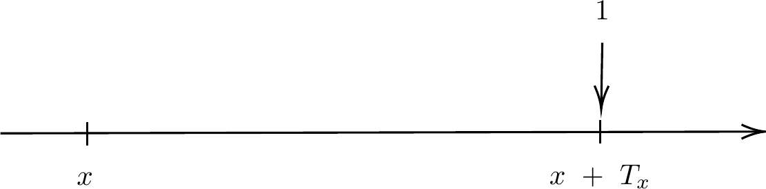
Fig. 15 The timeline of the whole life insurance contract

Tip

Further information can be found in the course Life Contingencies I.

The probability density function of \(T_x\)

The (remaining) future lifetime of a life aged \(x\) is a random variable \(T_x\), which is continuously distributed on an interval \([0,w], \, 0 < w < \infty\). The value \(w\) is called the limiting age, which is in practice taken the value in the range \([100,120]\). It is the maximum age beyond which it is not possible to live.

The distribution of \(T_x\) is

\[F_x(t) = \Pr(T_x \le t) = \Pr(\text{a life aged } (x) \text{ dies not later than } x+ t).\]

The survival function \(S_x(t)\) is defined as

\[S_x(t) = \Pr(T_x > t) = \Pr(\text{a life aged } (x) \text{ dies after (or survives to) age } x+ t).\]

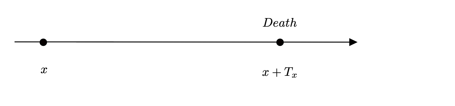
Fig. 16 Future life time random variable

These two functions define transition probabilities between Alive and Dead states in the mortality model (as given in the above diagram). Actuaries have their own notation as follows:

\[{}_{t}q_{x} = F_x(t) = \Pr(T_0 \le x + t | T_0 > x),\]

where \(T_0\) is the remaining future lifetime from birth. and

\[{}_{t}p_{x} = S_x(t) = \Pr(T_0 > x + t | T_0 > x) .\]

Force of mortality

The probability that a life alive at a given age will be dead at any subsequent age is governed by the force of mortality (or transition intensity or hazard rate or instantaneous rate of death). For age \(x\), \(0 \le x \le w\), we define

\[\mu_x = \lim_{h \rightarrow 0^+} \frac{1}{h} \times \Pr(T_0 \le x + h | T_0 > x).\]

It follows that for small \(h\), the transition probability \({}_{h}q_{x}\) can be approximated by

\[{}_{h}q_{x} \approx h \cdot \mu_x.\]

The force of mortality is measured with respect to a time unit. We will assume the time unit is year.

Example 3.26: Approximation of transition probability

Given that \(\mu_{70} \approx 0.05\) per year for males in Thailand, calculate approximately the probability that a 70 year old male dies within

(a) one day; (b) one week.

Solution to Example 3.26

Click to toggle answer

The transition probability \({}_{h}q_{x}\) can be approximated by

\[{}_{h}q_{x} \approx h \cdot \mu_x.\]

Hence,

\[{}_{\frac{1}{365}}q_{70} \approx \left( \frac{1}{365} \right) \times \mu_{70} = \left( \frac{1}{365} \right) \times 0.05 = 0.000137,\]

and

\[{}_{\frac{7}{365}}q_{70} \approx \left( \frac{7}{365} \right) \times \mu_{70} = \left( \frac{7}{365} \right) \times 0.05 = 0.000959.\]

Summary of model

• \(T_x\) is the (random) future lifetime after age \(x\). It is, by assumption, a continuous random variable taking values in \([0, \omega - x]\). Its distribution function is \(F_x(t) = {}_{t} q_x\).

• Its probability density function is \(f_x(t) = {}_{t}p_x \cdot \mu_{x+t}\).

• The force of mortality is interpreted by the approximate relationship: \({}_{h}q_x \approx h \cdot \mu_x\) (for small \(h\)).

• The survival functions \(S_x(t)\) or \({}_{t}p_x\) satisfy the relationship:

\[{}_{s+t}p_x = {}_{s}p_x \cdot {}_{t}p_{x + s} = {}_{t}p_x \cdot {}_{s}p_{x + t},\]

for any \(s > 0, t > 0.\)

Life Table

A life table is a statistical tool used to represent the mortality and survival patterns of a population. It organizes data on

• the probability of death and

• the number of survivors at each age for a given population over a specific period, typically one year.

Life tables are commonly used in demography, actuarial science, epidemiology, and public health to analyze population dynamics, forecast future trends, and calculate life expectancies.

Structure of a Life Table

1. Age: This signifies individual ages, often expressed as single years or grouped into intervals.

2. Expected Number of Deaths (\(d_x\)): This represents the expected number of individuals who die within the age interval, i.e. between the ages of \(x\) and \(x + 1\).

3. Expected Number of Lives (\(l_x\)): \(l_x\) denotes the expected number of lives at age \(x\)

4. Probability of Dying (\(q_x\)): This is the probability of dying within the specific age interval.

5. Life Expectancy (\(\mathring{e}_x\) (read “e-circle-x”)): This is the expected future lifetime after age \(x\) , which is referred to by demographers as the expectation of life at age \(x\).

Life table

The table represents the mortality rates of the population of England and Wales during the years 1990, 1991, and 1992.

We can observe the survival patterns, mortality rates, and life expectancies for different age groups within the population.

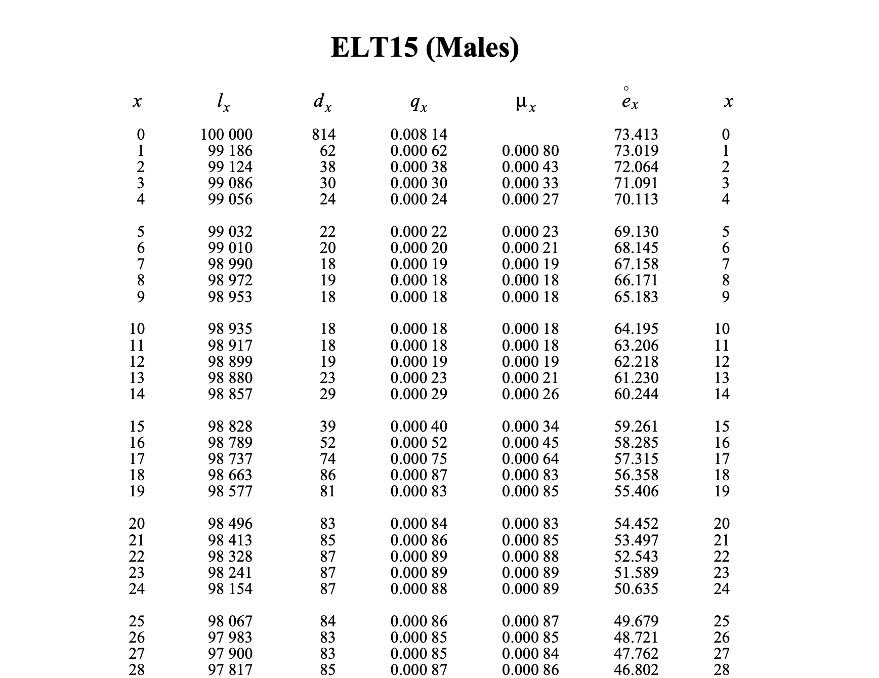
Fig. 17 The mortality of the population of England and Wales during the years 1990, 1991 and 1992

Tip

The survival and death probabilities can be calculated by the expected number of deaths and expected number of lives as follows:

\[\begin{split} \begin{align} d_x &= l_x - l_{x+1} \\ p_x &= \frac{l_{x+1}}{l_x} \\ q_x &= 1 - p_x = \frac{l_x - l_{x+1}}{l_x} = \frac{d_x}{l_x} \\ {}_{t}p_x &= \frac{l_{x+t}}{l_x} \\ {}_{t}q_x &= 1 - {}_{t}p_x = \frac{l_x - l_{x+t}}{l_x} \end{align} \end{split}\]

Example 3.27

Use the ELT15 (Males) table to calculate the following:

1. The probability that (50) survies to age 55.

2. The probability that (65) dies before age 70.

3. The probability that (70) dies before ages 75 and 80.

Solution to Example 3.27

Click to toggle answer

1. The probability of surviving from age 50 to age 55 is

\[{}_{5}p_{50} = \frac{l_{55}}{l_{50}} = 91217/93925 = 0.971168.\]

2. The probability that a life now aged 65 dies withing 5 years is

\[{}_{5}q_{65} = 1 - {}_{5}p_{65} = \frac{l_{65} - l_{70}}{l_{65}} = \frac{79293 - 68055}{79293} = 0.1417275.\]

3. The requied probability is the probability that a life now aged 70 dies between ages 75 and 80, denoted by \({}_{5|10}q_{70}\), which can be calculated by

\[\begin{split} \begin{align} {}_{5|10}q_{70} &= {}_{5}p_{70} - {}_{10}p_{70} \\ &= \frac{l_{75}}{l_{70}} - \frac{l_{80}}{l_{70}} \\ &= \frac{l_{75} - l_{80}}{l_{70}} \\ &= \frac{53266 - 36128}{68055} \\ &= 0.2518257 \end{align} \end{split}\]

The survival and death probabilities for a non-integer age

To find a value for a non-integer age, we need to make an assumption about how mortality changes between integer ages. One way to do this is to assume deaths happen evenly across the ages, or we could assume the mortality rate stays the same between whole ages.

Example 3.28: Estimation of the expected number of lives at a non-integer age

Based on the life table shown above, estimate \(l_{27.25}\), assuming a uniform distribution of deaths between exact ages 27 and 28.

Solution to Example 3.28

Click to toggle answer

The expected number of deaths between the ages of 27 and 29, \(d_{27}\), is given by

\[d_{27} = l_{27} - l_{28} = 97,900 - 97,817 = 83.\]

If we assume deaths are spread evenly throughout the year, we expect \(83/4 = 20.75\) deaths between ages 27 and 27.25. Therefore, the expected number of people alive at age 27.25 is 97,900 minus 20.75, which equals 97,879.25.

Complete expected future lifetime

Life Expectancy (\( E(T_x) = \mathring{e}_x \))

The life expectancy at age \( x \), denoted as \( \mathring{e}_x \), represents the expected number of years a person of age \( x \) is projected to live, on average. It is a crucial measure in actuarial science and demographic analysis, providing insight into population longevity and mortality trends.

Variance of Life Expectancy (Var(\( T_x \)))

The variance of life expectancy at age \( x \), denoted as \( \text{Var}(T_x) \), measures the dispersion or variability around the expected value \( \mathring{e}_x \). It indicates how much individual life expectancies at age \( x \) deviate from the average expectancy, offering insights into the uncertainty and risk associated with mortality projections.

Life Expectancy (\( E(T_x) = \mathring{e}_x \))

The life expectancy at age \( x \), denoted as \( \mathring{e}_x \), can be defined as the expected remaining lifetime for a person of age \( x \). Mathematically, it is represented as:

\[ E(T_x) = \mathring{e}_x = \int_{0}^{w-x} {}_{t}p_{x} \, dt \]

where:

• \( {}_{t}p_{x} \) denotes the probability that a person aged \( x \) survives to age \( x + t \),

• \( w \) is the limiting age, which is the maximum age up to which we are interested in calculating the life expectancy.

This integral represents the accumulation of survival probabilities from age \( x \) to age \( w \), providing an average estimation of remaining lifespan for individuals aged \( x \).

Variance of Life Expectancy (\( \text{Var}(T_x) \))

The variance of life expectancy at age \( x \), denoted as \( \text{Var}(T_x) \), measures the variability in the remaining lifetime for individuals aged \( x \). It can be defined as:

\[ \text{Var}(T_x) = \int_{0}^{w-x} t^2 ({}_{t}p_{x}) \mu_{x+t} \, dt - \left( \int_{0}^{w-x} {}_{t}p_{x} \, dt \right)^2 = 2 \int_{0}^{w-x} t ({}_{t}p_{x}) \, dt - (\mathring{e}_x)^2 \]

where:

• \( {}_{t}p_{x} \) denotes the probability that a person aged \( x \) survives to age \( x + t \),

• \( w \) is the limiting age, which is the maximum age up to which we are interested in calculating the life expectancy.

This expression represents the difference between the expected value of the square of remaining lifetimes and the square of the expected remaining lifetime. It quantifies the spread or dispersion of life expectancies around the mean expectancy, providing insights into the variability and risk associated with mortality projections.

Example 3.29: Complete expectation of life

Given \( S_0(x) = \left(1 - \frac{x}{120}\right)^{1/6} \) for \( 0 \le x \le 120\), calculate \(\mathring{e}_x\) and \( \text{Var}(T_x)\) for \(x = 20\) and \(x = 60\).

Solution to Example 3.29

Click to toggle answer

Calculation of \( E[T_x] \)

To find the life expectancy \( E[T_x] \) at age \( x \):

1. Survival Function:

\[ S_0(x) = \left(1 - \frac{x}{120}\right)^{1/6} \]

2. Probability of Survival:

\[ {}_{t}p_{x} = \frac{S_0(x+t)}{S_0(x)} = \left(\frac{1 - \frac{x+t}{120}}{1 - \frac{x}{120}}\right)^{1/6} = \left(1 - \frac{t}{120 - x}\right)^{1/6}\]

3. Integral for Life Expectancy:

\[ E[T_x] = \int_{0}^{120-x} {}_{t}p_{x} \, dt \]

4. Simplify the Integral: By making a substitution \( y = \left(1 - \frac{t}{120 - x}\right)\), it can be shown that

   \[ E[T_x] = \int_{0}^{120-x} \left(1 - \frac{t}{120 - x}\right)^{1/6} \, dt = \frac{6}{7} (120 - x)\]

This integral calculation provides the expected remaining lifetime for individuals aged \(x\), considering the given survival function.

Then \(\mathring{e}_{20} = 85.714\) and \(\mathring{e}_{60} = 51.429.\)

Calculation of \( \text{Var}(T_x) \)

By making a substition \( y = \left(1 - \frac{t}{120 - x}\right)\), it can be shown that

\[\begin{split} \begin{align} \text{Var}(T_x) &= 2 \int_{0}^{w-x} t ({}_{t}p_{x}) \, dt - (\mathring{e}_x)^2 \\ &= 2 \int_{0}^{w-x} t \left(1 - \frac{t}{120 - x}\right)^{1/6} \, dt - (\mathring{e}_x)^2 \\ &= 2(120 - x)^2 \left(\frac{6}{7} - \frac{6}{13} \right) - \left( \frac{6}{7} (120 - x) \right)^2 \end{align} \end{split}\]

Then \(\text{Var}(T_{20}) = 23.77^2\) and \(\text{Var}(T_{60}) = 14.26^2.\)

Curtate Expectation of Life

The curtate future lifetime of a life age \( x \), denoted by \( K_x \), is a random variable defined as the integer part of future lifetime as

\[ K_x = \lceil T_x \rceil, \]

where \( T_x \) represents the curtate future lifetime at age \( x \) and the square brackets denote the integer part. The curtate future lifetime \(K_x\) is the whole number of years lived after \( x \).

Curtate Expectation of Life

We now define the curtate expectation of life, denoted by \( e_x = E[K_x] \), as the expected number of years a person aged \( x \) is expected to live beyond their current age.

\[ e_x = E[K_x] = \sum_{k=0}^{\infty} {}_k p_x \]

Here, \( {}_k p_x \) denotes the curtate survival probability, which is the probability that a person aged \( x \) survives \( k \) years.

The variance of the curtate future lifetime is

\[ \text{Var}(K_x) = \sum_{k=0}^{\infty} k^2 {}_k p_x q_{x+k} - (e_x)^2 \]

Tip

The probability function of \(K_x\) is given by

\[ P(K_x = k) = {}_{k}p_{x} q_{x + k} \]

Example 3.30: Calculation of Expectations in Gompertz’s Survival Model

Calculate the complete and curtate expectations of life under Gompertz’s survival model with parameters \(B = 0.0003\) and \(c = 1.07\).

Solution to Example 3.30

Click to toggle answer

To calculate the complete and curtate expectations of life under Gompertz’s survival model with parameters \(B = 0.0003\) and \(c = 1.07\), follow these steps:

1. Gompertz’s Law Formula: Gompertz’s survival function is given by:

\[ {}_tp_x = \exp \left( - \frac{B}{\log c} (c^{x+t} - c^x) \right) \]

where:

• \( B \) is the Gompertz parameter related to the rate of aging,

• \( c \) is the shape parameter,

• \( x \) is the age.

2. Complete Expectation of Future Lifetime \( \mathring{e}_{x} \): The complete expectation of future lifetime \( e_x \) is calculated using:

\[ \mathring{e}_{x} = \int_0^{\infty} {}_tp_x \, dt \]

First, we simplify the exponent:

\[ \exp\left(- \frac{B}{\log(c)} (c^{x+t} - c^x) \right) \]

Simplify the term inside the exponent:

\[ \frac{B}{\log(c)} (c^{x+t} - c^x) \]

Let \( k = \frac{B}{\log(c)} \), then the term becomes:

\[ k (c^{x+t} - c^x) \]

Let’s define a new variable \( u = c^t \), which means \( du = c^t \log(c) dt \) or \( dt = \frac{du}{u \log(c)} \).

The integral bounds change from \( t \in [0, \infty) \) to \( u \in [1, \infty) \).

The integral becomes:

\[ \int_{1}^{\infty} \exp\left(- k (c^x u - c^x) \right) \frac{du}{u \log(c)} \]

Simplify the exponent:

\[ \exp\left(- k c^x (u - 1) \right) \]

The integral is now:

\[ \int_{1}^{\infty} \exp\left(- k c^x (u - 1) \right) \frac{du}{u \log(c)} \]

We can now evaluate this integral numerically using a different approach to avoid overflow.

Let’s compute this integral using Python:

import numpy as np
from scipy.integrate import quad

# Constants
B = 0.0003
c = 1.07
x = 10  # Example value for x, you can modify it as needed

# Define the integrand with the new variable u
def integrand(u):
    k = B / np.log(c)
    return np.exp(- k * c ** x * (u - 1)) / (u * np.log(c))

# Compute the integral
result, error = quad(integrand, 1, np.inf)

result, error

(62.22279284724417, 3.807848119729502e-08)

Let us iterate over the values of \(x\) from 0 to 100 in steps of 10 and compute the integral for each value. Here is the Python code to perform the integration and print out the results:

import numpy as np
from scipy.integrate import quad

# Constants
B = 0.0003
c = 1.07

# Define the integrand with the new variable u
def integrand(u, x):
    k = B / np.log(c)
    return np.exp(- k * c ** x * (u - 1)) / (u * np.log(c))

# Values of x
x_values = range(0, 101, 10)

# Compute the integral for each value of x and print the results
for x in x_values:
    result, error = quad(integrand, 1, np.inf, args=(x,))
    print(f"x = {x}: integral = {result}, error = {error}")

x = 0: integral = 71.93751321477427, error = 3.449608108160561e-08
x = 10: integral = 62.22279284724417, error = 3.807848119729502e-08
x = 20: integral = 52.70287730280692, error = 4.02435489448526e-08
x = 30: integral = 43.49195898800364, error = 4.058528995119045e-08
x = 40: integral = 34.751553038275816, error = 3.884354401415047e-08
x = 50: integral = 26.691143608815153, error = 3.494671597890118e-08
x = 60: integral = 19.550450161058592, error = 2.8908359439274028e-08
x = 70: integral = 13.554854033123279, error = 2.0319647530398746e-08
x = 80: integral = 8.84844789828676, error = 6.961164407463761e-09
x = 90: integral = 5.43256409984473, error = 2.6496040228513092e-08
x = 100: integral = 3.1515686655638433, error = 2.3989044503723047e-09

Solution to Example 3.30 (cont.)

Click to toggle answer

3. Curtate Expectation of Life \( e_x \): The curtate expectation of life \( K_x \) is computed as:

   \[ e_x = \sum_{k=0}^{\infty} {}_k p_x \]

   where \( {}_k p_x \) represents the curtate survival probability at age \( x \).

To proceed, substitute the values \( B = 0.0003 \) and \( c = 1.07 \) into the respective formulas to determine \( \mathring{e}_{x} \) and \( e_x \).

Let’s compute this integral using Python:

import numpy as np

# Constants
B = 0.0003
c = 1.07
x = 10

# Define the survival probability function
def survival_probability(k, x):
    return np.exp(- (B / np.log(c)) * (c**(x+k) - c**x))

# Compute the Curtate Expectation of Life e_x
def curtate_expectation_of_life(x, max_k=1000):
    return sum(survival_probability(k, x) for k in range(max_k))

# Compute e_x for x = 10
e_x = curtate_expectation_of_life(x)
print(f"e_{x} = {e_x}")

e_10 = 62.72284202237426

The relationship between the complete and curtate expectations of life

Alternatively, the complete and curtate expectations of life are related by the approximate equation:

\[ \mathring{e}_{x} \approx e_x + \frac{1}{2} \]

where \( \mathring{e}_{x} \) represents the complete expectation of life and \(e_x\) represents the curtate expectation of life.

Actuarial Models in Life Insurance: Whole life assurance contracts Payable at the End of the Year of Death

Whole life assurance contracts are a type of life insurance that guarantees a payout to the policyholder’s beneficiaries upon the policyholder’s death. Understanding the expected present value and its variability is crucial for both insurance providers and policyholders.

In what follows, we will focus on the whole life assurance contracts payable at the end of the year of death. This timeline visually demonstrates the conditions of whole life insurance, where the death benefit is guaranteed and payable at the end of the year of the death of the insured individual.

Let us explore the key concepts and calculations associated with these contracts, where we set out the basic equation of value for an insurance contract.

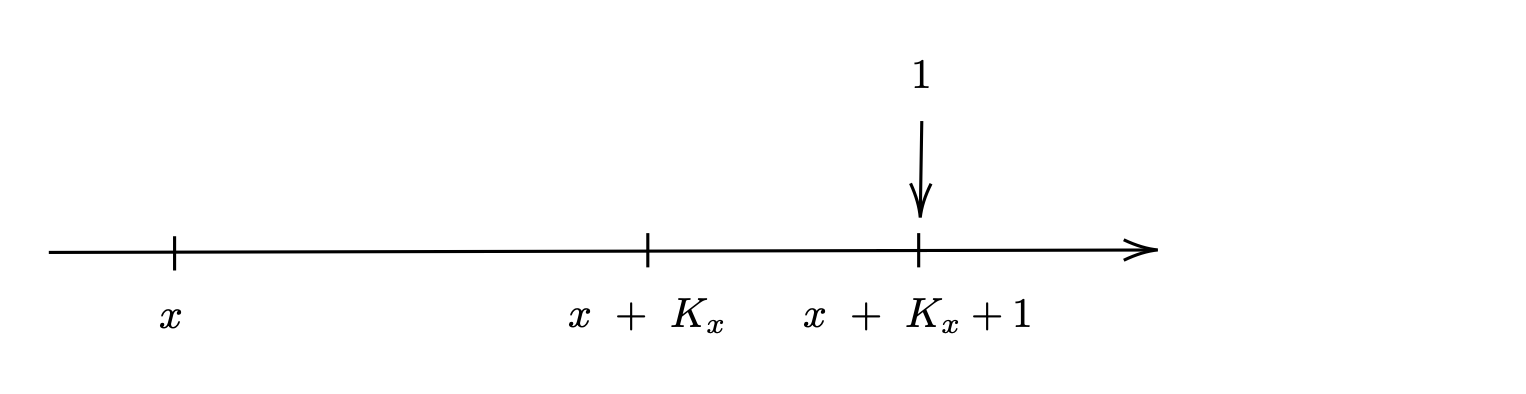
Fig. 18 The timeline of the whole life insurance contract

Expected Present Value (EPV) of this whole life assurance

The expected present value (EPV) refers to the present value of a payment that is contingent upon an uncertain future event—in this case, the death of the policyholder.

Simple Whole Life Assurance Contract

A simple whole life assurance contract pays a sum assured (\(S\)) to the beneficiaries at the end of the year of the death.

Present Value Random Variable

For a whole life assurance contract, the time of payment (\(K_x + 1\)) is uncertain because we do not know when the policyholder will die. Here, \(K_x\) represents the number of complete years a person of age \(x\) survives before dying.

Conventions

1. Convention 1: The benefit is considered for a person currently aged \(x\) (an integer).

2. Convention 2: The sum assured (\(S\)) is payable at the end of the year of death.

Under these conventions, the sum assured \(S\) will be paid at time \(K_x + 1\). We use the notation \((x)\) to denote a person currently aged \(x\).

Expected Present Value (EPV) of this whole life assurance Suppose that the rate of interest is \(i\) per year. Let \(v = 1/(1+i)\). The expected value of \(S v^{K_x+1}\), denoted as \(E[S v^{K_x+1}]\), represents the average present value of the benefit over all possible scenarios of the policyholder’s death.

\[E[S v^{K_x+1}] = S \sum_{k=0}^\infty v^{k+1} P(K_x = k) = S \sum_{k=0}^\infty v^{k+1} {}_{k}p_{x} \cdot q_{x + k}\]

Denote \(A_x = E[v^{K_x+1}]\).

Variance The variance of \(S v^{K_x+1}\), denoted as \(Var[S v^{K_x+1}]\), measures the variability or risk associated with the present value of the benefit.

\(Var[S v^{K_x+1}] = S^2 Var[v^{K_x+1}] = S^2 (^2A_x - (A_x)^2) \)

where \(^2A_x\) is the expected present value of a whole life insurance calculated at a rate of interest of \(i_2 = 2i + i^2.\)

Example 3.31: Calculation of Expectations of a Whole Life Insurance in Gompertz’s Survival Model

A survival model follows Gompertz’s survival model with parameters \(B = 0.0003\) and \(c = 1.07\). Calculate the Expected Present Value (EPV) of the whole life assurance, \(A_x\) and the standard deviation of \(v^{K_x+1}\) assuming that the rate of interest is 5%.