Exercises for Chapter 2.3#
Exercise 2.13
Explain the properties of the probability mass function (PMF) of a discrete random variable.
Solution to Exercise 2.13
Click to toggle answer
The probability mass function (PMF) of a discrete random variable has several key properties
Non-negativity
The PMF is non-negative for all possible values of the random variable.
Summation to One
The sum of probabilities over all possible values of the random variable equals one
Probability Distribution
Each value in the range of the random variable has a corresponding probability that represents the likelihood of that value occurring.
Ranges and Bounds
The PMF defines the probability of each individual outcome in the sample space of the random variable.
Discrete Nature
Since it’s defined for discrete random variables, the PMF assigns probabilities to individual outcomes rather than ranges of outcomes.
Point Probabilities
The PMF gives the probability of a specific value occurring for the discrete random variable.
Cumulative Distribution Function (CDF)
The cumulative distribution function (CDF) can be derived from the PMF. It represents the probability that the random variable takes on a value less than or equal to a given value.
Exercise 2.14
Explain the properties of the probability density function (PDF) of a continuous random variable.
Solution to Exercise 2.14
Click to toggle answer
Non-negativity
The PDF is non-negative for all values of the random variable.
Area under the Curve
The total area under the PDF curve over its entire domain is equal to one:
\[ \int_{-\infty}^{\infty} f(x) \, dx = 1 \]This property ensures that the total probability of all possible outcomes is one.
Probability at a Single Point
The probability of a continuous random variable taking on a specific value is zero:
This is because the PDF represents a continuous distribution, and the probability of any single point in a continuous distribution is infinitesimally small.
Probability within an Interval
The probability of a continuous random variable falling within a certain interval is given by the area under the PDF curve over that interval:
This reflects the likelihood of the random variable taking on values within the specified range.
Relative Likelihood
The height of the PDF at any point represents the relative likelihood of the random variable taking on values near that point.
Smoothness
The PDF is a smooth function, indicating that there are no abrupt changes or discontinuities in the probability distribution.
Derivation of Cumulative Distribution Function (CDF)
The cumulative distribution function (CDF) of the continuous random variable can be derived by integrating the PDF:
\[ F(x) = \int_{-\infty}^{x} f(t) \, dt \]This function gives the probability that the random variable is less than or equal to a given value.
Exercise 2.14
How can we use R to visually explore the probability mass function (PMF) and cumulative distribution function (CDF) of the Poisson distribution for three distinct parameters \(\lambda\)? Use Wikipedia as a reference for an example. Please ensure to provide appropriate titles, legends, and axis labels for clarity.
Exercise 2.15
How can we use R to visually explore the probability mass function (PMF) and cumulative distribution function (CDF) of the following distributions
Binomial,
Normal,
Exponential, and
Gamma,
across various parameters? Using Wikipedia as a reference for examples, please ensure to include appropriate titles, legends, and axis labels for clarity in the plots.
Exercise 2.16
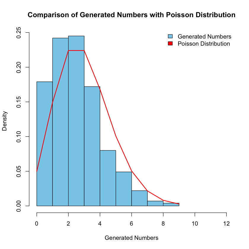
How can we use R to explore the Poisson distribution with a parameter of our choice? Let’s select a parameter and generate random numbers from this Poisson distribution. Afterward, let’s discuss how we can visualize and compare the generated numbers with the Poisson distribution to gain insights into their distribution characteristics.
Solution to Exercise 2.16
Here’s the R code to accomplish the tasks:
# Define the parameter for the Poisson distribution
lambda <- 3

# Generate random numbers from the Poisson distribution
nsample <- 1000
random_numbers <- rpois(nsample, lambda)

# Visualize the generated numbers and compare with the Poisson distribution
hist(random_numbers, freq = FALSE, col = "skyblue", main = "Comparison of Generated Numbers with Poisson Distribution",
     xlab = "Generated Numbers", ylab = "Density", xlim = c(0, max(random_numbers)+3))

# Add the Poisson distribution curve
x <- 0:max(random_numbers)  # Possible values for Poisson distribution
lines(x, dpois(x, lambda), type = "l", col = "red", lwd = 2)
legend("topright", legend = c("Generated Numbers", "Poisson Distribution"), fill = c("skyblue", "red"), bty = "n")
Exercise 2.17
How can we use R to explore the following distributions
Binomial,
Normal,
Exponential, and
Gamma,
with parameters of our choice? Let’s select parameters and generate random numbers from each of these distributions. Afterward, let’s discuss how we can visualize and compare the generated numbers with their respective distributions to gain insights into their distribution characteristics.