3.4 Cashflows and Annuities#
In this section, we will explore the basics of cashflows, how money moves over time, and what factors affect it. We will also break down annuities, which are financial tools designed to provide a steady income for a specific period.
Definitions
(1) Cashflows refer to the movement of money into or out of a business, investment, or financial instrument over a specific period. They can be either positive (inflows) when money is received, or negative (outflows) when money is paid out.
Understanding cashflows is crucial in financial analysis as they reflect the liquidity and financial health of an entity.
(2) Annuities are financial products typically offered by insurance companies, structured to provide a series of payments at regular intervals, usually monthly, quarterly, or annually, in exchange for a lump sum payment or a series of payments made over time.
They are commonly used as retirement income vehicles but can also serve other purposes such as structured settlements or funding for education.
Classification of Annuities
Based on Payment Structure
Immediate Annuities: Immediate annuities begin providing payments to the annuitant shortly after the initial investment, usually within a year. They are often purchased with a lump sum and offer immediate income for a specified period or for life.
Deferred Annuities: Deferred annuities delay payments until a future date chosen by the annuitant, allowing the initial investment to grow tax-deferred until withdrawals begin. They can be fixed, variable, or indexed, offering flexibility in investment choices and payout options.
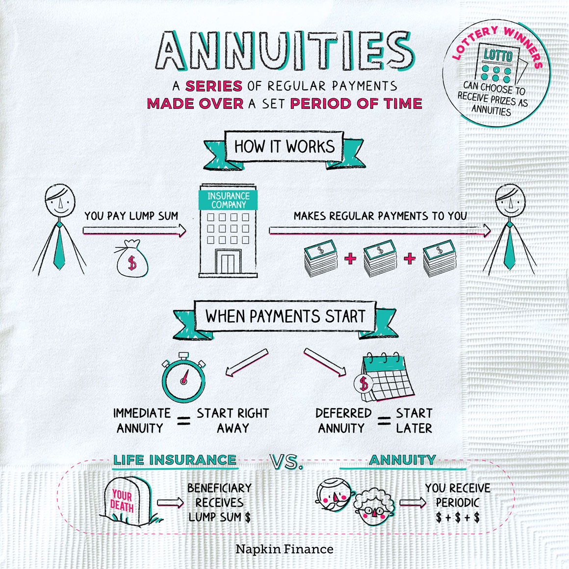
Fig. 11 Image from https://napkinfinance.com/napkin/annuities/#
Classification of Annuities
Based on Timing of Payments
Ordinary Annuity (or Annuity in Arrears)
Payments are made at the end of each period, after the period has elapsed.
Commonly seen in loans, mortgages, and some retirement plans.
Annuity Due
Start making payments immediately after the initial investment.
Payments are made at the beginning of each period.
Based on Payment Structure
Level Annuities (or Fixed Annuities)
Offer a constant stream of payments throughout the annuity period.
Payments remain the same over time, providing predictability to the annuitant.
Increasing Annuities (or Escalating Annuities)
Provide payments that gradually increase over time, typically to account for inflation or changing needs of the annuitant.
Decreasing Annuities
Offer payments that decrease over time, often chosen when the annuitant expects their expenses to decrease, such as in retirement.
Present Value and Future Value of Cash Flows and Annuities#
Present Value of Annuities (PVA) Present value of annuities is the current worth of a series of future cash flows received or paid at regular intervals, discounted at the effective rate of interest.
Future Value of Annuities (FVA) Future value of annuities is the value of a series of equal payments or cash flows received or paid at regular intervals, compounded at the effective rate of interest to a specified future date.
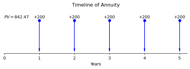
Example 3.21: Present Value of Annuities (\(PV A\)) Example
Suppose you have an annuity that pays $200 at the end of each year for 5 years, and the effective annual interest rate is 6%. You want to calculate the present value of this annuity.
Using the present value of annuities formula:
Where:
\(PVA\) = Present Value of Annuities
\(PMT\) = Payment per period ($200 in this case)
\(i\) = Effective rate of interest per period (6% in this case)
\(n\) = Number of periods (5 years in this case)
Substituting the values:
Interpretation: The present value of receiving $200 at the end of each year for 5 years, with an effective annual interest rate of 6%, is approximately $842.47.
Show code cell source
import numpy as np
import matplotlib.pyplot as plt
%matplotlib inline

# Parameters
payment = 200
years = 5
interest_rate = 0.06

# Compute present value
present_value = np.sum([payment / (1 + interest_rate)**i for i in range(1, years + 1)])

# Plotting
plt.figure(figsize=(8, 1.5))  # Adjusted width to 2 cm

# Adding arrows
for i in range(1, years + 1):
    plt.arrow(i, payment, 0, -payment * 0.9, head_width=0.03, head_length=payment * 0.1, fc='blue', ec='blue')

# Adjusted x and y data to remove dot at 0
plt.plot([i for i in range(1, years + 1)], [payment]*years, marker='o', linestyle='', color='b')

# Adjusted text position
for i in range(1, years + 1):
    plt.text(i, payment + 10, f'+{payment}', verticalalignment='bottom', horizontalalignment='center')

plt.xlabel('Years')
plt.ylabel('Cash Flow ($)')
plt.title('Timeline of Annuity', y=1.3)  # Adding small space above the figure
plt.xticks(np.arange(0, years + 1, 1))
plt.grid(False)
plt.gca().spines['top'].set_visible(False)
plt.gca().spines['right'].set_visible(False)
plt.gca().spines['left'].set_visible(False)
plt.gca().get_yaxis().set_visible(False)


# Adjusted text position
plt.text(0, payment + 10, f'$PV = {present_value:.2f}$', verticalalignment='bottom', horizontalalignment='left')

plt.show()
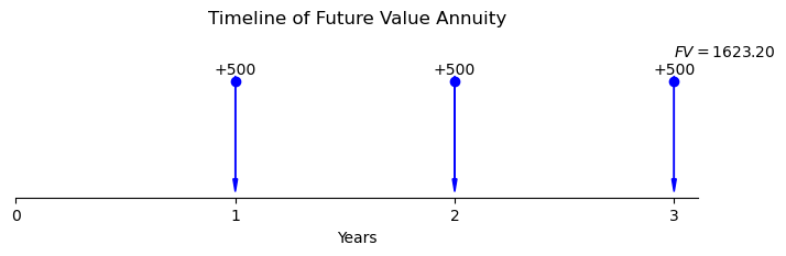
Example 3.22: Future Value of Annuities (\(FV A\)) Example
Suppose you invest $500 at the end of each year for 3 years in an account with an effective annual interest rate of 8%. You want to calculate the future value of this annuity.
Using the future value of annuities formula:
Where:
\(FVA\) = Future Value of Annuities
\(PMT\) = Payment per period ($500 in this case)
\(i\) = Effective rate of interest per period (8% in this case)
\(n\) = Number of periods (3 years in this case)
Substituting the values:
Interpretation: The future value of investing $500 at the end of each year for 3 years, with an effective annual interest rate of 8%, will be approximately $1,623.20.
Show code cell source
import numpy as np
import matplotlib.pyplot as plt
%matplotlib inline

# Parameters
investment = 500
years = 3
interest_rate = 0.08

# Compute future value
future_value = np.sum([investment * (1 + interest_rate)**i for i in range(years)])

# Plotting
plt.figure(figsize=(8, 1.5))  # Adjusted height to 2 cm

# Adding arrows
for i in range(1, years + 1):
    plt.arrow(i, investment, 0, -investment * 0.8 , head_width=0.02, head_length=investment * 0.1, fc='blue', ec='blue')

# Adjusted y-coordinate for the dots and text
plt.plot([i for i in range(1, years + 1)], [investment - 20]*years, marker='o', linestyle='', color='b')

for i in range(1, years + 1):
    plt.text(i, investment - 5, f'+{investment}', verticalalignment='bottom', horizontalalignment='center')

plt.xlabel('Years')
plt.ylabel('Cash Flow ($)')
plt.title('Timeline of Future Value Annuity', y=1.3)
plt.xticks(np.arange(0, years + 1, 1))
plt.grid(False)
plt.gca().spines['top'].set_visible(False)
plt.gca().spines['right'].set_visible(False)
plt.gca().spines['left'].set_visible(False)
plt.gca().get_yaxis().set_visible(False)

plt.text(3, investment + 65, f'$FV = {future_value:.2f}$', verticalalignment='bottom', horizontalalignment='left')

plt.show()
Actuarial Notation for Annuities#
In actuarial science, the present value and future value of annuities are often represented using specific notation. This notation helps actuaries and financial professionals to succinctly express these calculations.
The expression \(a_{\overline{n|}i}\)
The expression \(a_{\overline{n|}i}\) (read a-angle-n at i) denotes the present value of an annuity-immediate, which is a series of unit payments at the end of each year for \(n\) years. Mathematically, it represents the sum of the present values of these unit payments.
The formula to calculate \(a_{\overline{n|}i}\) is:
where:
\(v\) is the discount factor for one period (often denoted as \(\frac{1}{1+i}\), where \(i\) is the interest rate or discount rate).
\(n\) is the number of periods (years in this case).
\(i\) is the interest rate or discount rate.
So, \(a_{\overline{n|}i}\) represents the present value of receiving \(n\) unit payments at the end of each year, discounted at an interest rate \(i\). It’s essentially the sum of a geometric series of payments.
The expression \(s_{\overline{n|}i}\)
The expression \(s_{\overline{n|}i}\) (read s-angle-n at i) represents the value at the time of the last payment of an annuity-immediate, which is a series of unit payments at the end of each year for \(n\) years. This value is obtained from:
where:
\(v\) is the discount factor for one period (often denoted as \(\frac{1}{1+i}\), where \(i\) is the interest rate or discount rate).
\(n\) is the number of periods (years in this case).
\(i\) is the interest rate or discount rate.
So, \(s_{\overline{n|}i}\) represents the value at the time of the last payment of an annuity-immediate, discounted at an interest rate \(i\). It’s essentially the sum of a geometric series of payments plus the initial payment at time 0.
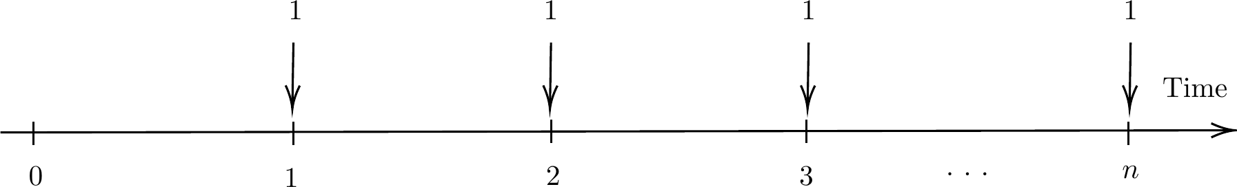
Fig. 12 A series of unit payments at the end of each year for \(n\) years#
Present Value of Annuities#
The present value of annuities represents the current worth of a series of future cash flows received or paid at regular intervals, discounted at a specified interest rate.
Formula for the present value of annuities
The formula for the present value of annuities is expressed as:
Where:
\(PV\) = Present Value of Annuities with \(n\) payments at an interest rate of \(i\)
\(PMT\) = Payment per period
\(i\) = Interest rate per period
\(n\) = Number of periods
\(v\) = The discount factor for one period (often denoted as \(\frac{1}{1+i}\), where \(i\) is the interest rate or discount rate).
Future Value of Annuities#
The future value of annuities represents the value of a series of equal payments or cash flows received or paid at regular intervals, compounded at a specified interest rate to a future date.
Formula for the future value of annuities
The formula for the future value of annuities is expressed as:
Where:
\(FV\) = Future Value of Annuities with \(n\) payments at an interest rate of \(i\)
\(PMT\) = Payment per period
\(i\) = Interest rate per period
\(n\) = Number of periods
These notations are commonly used in actuarial calculations and financial analysis to represent the present and future values of annuities.
Example 3.23: Present and Future Values of Annuities
Given the effective rate of interest of \(8\%\) p.a., calculate
the accumulation at 12 years of ฿500 payable yearly in arrears for the next 12 years.
the present value now of ฿2,000 payable yearly in arrears for the next 6 years.
the present value now of ฿1,000 payable half-yearly in arrears for the next 12.5 years.
Solution to Example 3.23
Click to toggle answer
The accumulation of the payments is
The present value of the payments is
An interest rate of 8% p.a. is equivalent to an effective half-yearly interest rate, denoted by \(j\), of
There are 25 payments of 1000 each, starting in six months’ time.
Working in terms of half year, the present value of the payment is
Importance of Calculating the Present and Future Value of Annuities#
Calculating the present value (PV) and future value (FV) of annuities is essential for several reasons:
Financial Planning: PV and FV calculations help individuals and businesses in financial planning. By knowing the present and future worth of annuities, they can make informed decisions about saving, investing, borrowing, or lending money.
Investment Analysis: Investors use PV and FV calculations to evaluate the attractiveness of investment opportunities. Comparing the present value of expected cash flows (such as dividends or interest payments) to the initial investment helps determine the profitability of an investment.
Budgeting: Understanding the present value of annuities allows individuals to budget their finances effectively. It helps them plan for regular expenses or income streams, ensuring financial stability over time.
Loan and Mortgage Decisions: Lenders and borrowers use PV and FV calculations to assess the affordability and terms of loans or mortgages. Knowing the present value of loan payments helps borrowers understand the total cost of borrowing, while lenders can determine the profitability of lending.
Retirement Planning: For retirement planning, individuals need to calculate the future value of annuities to ensure they have sufficient funds to maintain their desired lifestyle after retirement. Knowing the future value helps them set savings goals and make contributions to retirement accounts accordingly.
Insurance Planning: Insurance companies use PV and FV calculations to determine premiums and payouts for annuity products. Understanding the present and future value of annuities helps insurers manage risk and ensure they can meet their financial obligations to policyholders.
Overall, calculating the present and future value of annuities provides valuable insights into the timing and magnitude of cash flows, enabling better financial decision-making and planning for both individuals and businesses.