Chapter 6 Tutorials
6.1 Tutorial 1
- Using the method of moments, calculate the parameter values for the gamma, lognormal and Pareto distributions for which \[\mathrm{E}[X] = 500 \quad \text{and} \quad \mathrm{Var}[X] = 100^2.\] Answer:
gamma: \(\tilde{\alpha} = 25\), \(\tilde{\lambda} = 0.05.\)
lognormal: \(\tilde{\mu} = 6.194998\), \(\tilde{\sigma} = 0.1980422.\)
the MME cannot apply for the Pareto distribution. For the given values of \[\mathrm{E}[X] = 500 \quad \text{and} \quad \mathrm{Var}[X] = 100^2\], the obtained values of \(\tilde{\alpha}\) and \(\tilde{\lambda}\) from the method of moments are negative. Note that if we fix \(s = 100^2\) and vary \(\bar{x}\) within the interval \([90,110]\), the plot of \(\bar{x}\) against \(\tilde{\alpha}\) is shown below. Notice that when \(\bar{x} = 100\), \(\tilde{\alpha}\) tends to infinity.
xbar <-90:110
s <- 100
# MME
alpha_tilde <- 2*s^2/xbar^2 * 1/(s^2/xbar^2 - 1)
lambda_tilde <- xbar*(alpha_tilde -1)
plot(xbar,alpha_tilde, xlab = expression(bar(x)), ylab = expression(alpha))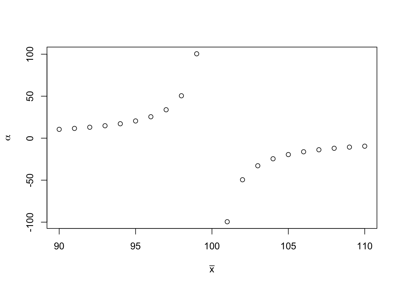
- Show that if \(X \sim \text{Exp}(\lambda)\), then the random variable \(X-w\) conditional on \(X > w\) has the same distribution as \(X\), i.e. \[X \sim \text{Exp}(\lambda)\Rightarrow X - w | X > w \sim \text{Exp}(\lambda).\]
Solution: Let \(W = Z|Z>0\) be a random variable representing the amount of a non-zero payment by the reinsurer on a reinsurance claim. The distribution and density of \(W\) can be calculated as follows: for \(x > 0\), \[ \begin{aligned} \Pr[W \le x ] &= \Pr[Z \le x | Z >0] \\ &= \Pr[X - M \le x | X > M] \\ &= \frac{\Pr[M < X \le x + M]}{\Pr[X > M]}\\ &= \frac{F_X(x+M) - F_X(M)}{1-F_X(M)}. \end{aligned} \]
Given \(X \sim \textrm{Exp}(\lambda)\), \(F_X(x) = 1 - e^{-\lambda x}.\) Moreover,
\[ \begin{aligned} \Pr[W \le x ] &= \frac{F_X(x+M) - F_X(M)}{1-F_X(M)} \\ &= \frac{ e^{-\lambda (M)} - e^{-\lambda (x+M)}}{e^{-\lambda (M)}} \\ &= 1 - e^{-\lambda x}. \end{aligned} \] Hence, \(W \sim \textrm{Exp}(\lambda)\).
- Derive an expression for the variance of the \(\text{Pa}(\alpha, \lambda)\) distribution. (Hint: using the pdf)
Solution: Recall that that for \(X \sim \mathcal{Pa}(\alpha,\lambda)\), its density function is \[ f_X(x) = \frac{\alpha \lambda^\alpha}{ (x + \lambda)^{\alpha + 1}}.\] \[ \begin{aligned} \mathrm{E}[X] &= \int_0^\infty x \frac{\alpha \lambda^\alpha}{ (x + \lambda)^{\alpha + 1}}\, dx \quad \text{(using integration by part:} \quad u = x \text{ and } (\lambda + x)^{-(\alpha + 1)}dx = dv) \\ &= -\alpha \lambda^\alpha \left( \frac{x}{\alpha} (\lambda + x)^{-\alpha} \right)\bigg|_0^\infty + (\alpha \lambda^\alpha)(\frac{1}{\alpha})\int_0^\infty \frac{1}{(\lambda + x)^\alpha} \, dx \end{aligned} \] Using the fact that for \(X \sim \mathcal{Pa}(\alpha,\lambda)\), \(\textrm{E}[X]\) exists when \(\alpha > 1\), which will be assumed on the first term above. This assumption simplifies the above results as follows:
\[ \begin{aligned} \mathrm{E}[X] &= 0 + \int_0^\infty \frac{\lambda^\alpha}{(\lambda + x)^\alpha} \, dx \\ &= \frac{\lambda}{\alpha - 1} \int_0^\infty \frac{(\alpha - 1)\lambda^{\alpha - 1}}{(\lambda + x)^\alpha} \, dx \\ &= \frac{\lambda}{\alpha - 1} \cdot 1. \end{aligned} \] Note that the last integral integrate to 1 because the integrand is the density function of a Pareto distribution.
One can also show that \[ \mathrm{E}[X^2] = \frac{2 \lambda^2}{(\alpha - 1)(\alpha - 2)}.\] Therefore, \[ \mathrm{Var}[X] = \mathrm{E}[X^2] - (\mathrm{E}[X])^2 = \frac{\alpha \lambda^2}{(\alpha - 1)^2(\alpha - 2)}.\]
Show that the MLE (the maximum likelihood estimation) of \(\lambda\) for an \(\text{Exp}(\lambda)\) distribution is the reciprocal of the sample mean, i.e. \(\hat\lambda = 1/ \bar x\). Solution: Suppose we have a random sample \(x = (x_1, x_2, \ldots, x_n)\) of \(X \sim \text{Exp}(\lambda).\) We have \[ \begin{aligned} L(\lambda) &= \Pi_{i=1}^n f(x_i, \lambda) = \Pi_{i=1}^n \lambda e^{-\lambda x_i} = \lambda^n e^{-\lambda \sum x_i}. \\ l(\lambda) &= \log( L(\lambda)) = n \log(\lambda) - \lambda \sum x_i \end{aligned} \] The MLE can be obtained by maximise \(l(\lambda)\) with respect to \(\lambda\). \[ \frac{d\, l(\lambda)}{d \lambda } = \frac{n}{\lambda} - \sum x_i = 0. \] Therefore, the MLE of \(\lambda\) is \(\hat{\lambda} = 1/\bar{x}.\)
Claims last year on a portfolio of policies of a risk had a lognormal distribution with parameter \(\mu = 5\) and \(\sigma^2 = 0.4\). It is estimated that all claims will increase by 15% next year. Find the probability that a claim next year will exceed 1000. Solution: From \(X \sim \mathcal{LN}(5,0.4)\), \(\log X \sim \mathcal{N}(5,0.4)\). Claims in next year will increase by 15%. We define \(Y = (1+15\%) X = 1.15 X\). We also have \[ \begin{aligned} \Pr(Y > 1000) &=\Pr(1.15 X > 1000) \\ &=\Pr(\log X > \log (1000/1.15)) \\ &=\Pr\left(Z > \frac{\log (1000/1.15)) - 5 }{\sqrt{0.4}}\right) \\ &=\Pr\left(Z > 2.7954\right) \\ &=1 - \Pr\left(Z \le 2.7954\right) \\ &= 1 - 0.9974082 = 0.002591777. \\ \end{aligned} \] I used
Rto obtain the required probability.
6.2 Tutorial 2
Claims occur on a general insurance portfolio independently and at random. Each claim is classified as being of “Type A” or “Type B”. Type A claim amounts are distributed \(\text{Pa}(3,400)\) and Type B claim amounts are distributed \(\text{Pa}(4,1000)\). It is known that 90% of all claims are of Type A.
Let \(X\) denote a claim chosen at random from the portfolio.
Calculate \(\Pr(X > 1000).\)
Calculate \(\mathrm{E}[X]\) and \(\mathrm{Var}[X]\).
Let \(Y\) have a Pareto distribution with the same mean and variance as \(X\). Calculate \(\Pr(Y > 1000).\)
Comment on the difference in the answers found in 1.1 and 1.2.
An insurer covers an individual loss \(X\) with excess of loss reinsurance with retention level \(M\). Let \(Y\) and \(Z\) be random variables representing the amounts paid by the insurer and reinsurer, respectively, i.e. \(X = Y + Z\). Show that \(\mathrm{Cov}[Y,Z] \ge 0\) and deduce that \[\mathrm{Var}[X] \ge \mathrm{Var}[Y] + \mathrm{Var}[Z].\] Comment on the results obtained.
Claim amounts from a general insurance portfolio are lognormally distributed with mean 200 and variance 2916. Excess of loss reinsurance with retenton level 250 is arranged. Calculate the probability that the reinsurer is involved in a claim.
Show that if \(X \sim \text{Pa}(\alpha, \lambda)\), then the random variable \(X-d\) conditional on \(X > d\) has a pareto distribution with parameters \(\alpha\) and \(\lambda + d\), i.e. \[X \sim \text{Pa}(\alpha, \lambda)\Rightarrow X - d | X > d \sim \text{Pa}(\alpha,\lambda + d).\]
Consider a portfolio of motor insurance policies. In the event of an accident, the cost of the repairs to a car has a Pareto distribution with parameters \(\alpha\) and \(\lambda\). A deductible of 100 is applied to all claims and a claim is always made if the cost of the repairs exceeds this amount. A sample of 100 claims has mean 200 and standard deviation 250.
Using the method of moments, estimate \(\alpha\) and \(\lambda\).
Estimate the proportion of accidents that do not result in a claim being made.
The insurance company arranges excess of loss reinsurance with another insurance company to reduce the mean amount it pays on a claim to 160. Calculate the retention limit needed to achieve this.
6.3 Solutions to Tutorial 2
Solution:
\[\begin{aligned} \Pr(X > 1000) &= \Pr(X > 1000 | A) \Pr(A) + \Pr(X > 1000 | B) \Pr(B) \\ &= \left( \frac{ 400 }{ 1000 + 400} \right)^{3} (0.9) + \left( \frac{ 1000 }{ 1000 + 1000} \right)^{4} (0.1) \\ &= 0.0272413. \end{aligned}\]
Using the conditional expectation and conditional variance formulas, we have
\[\begin{aligned} \mathrm{E}[X|A] &= \frac{400 }{3 - 1} = 200, \\ \mathrm{E}[X|B] &= \frac{1000 }{4 - 1} = 333.3333333. \end{aligned} \] Hence, \[\begin{aligned} \mathrm{E}[X] &= \mathrm{E}[\mathrm{E}[X|\text{type}]] \\ &= \Pr(A) \, \mathrm{E}[X|A] + \Pr(B) \, \mathrm{E}[X|B] \\ &= (0.9)(200) + (0.1)(333.3333333) \\ &= 213.3333333. \end{aligned} \]
We also have\[\begin{aligned} \mathrm{E}[X^2|A] &= \mathrm{Var}[X|A] + (\mathrm{E}[X|A])^2 = \frac{(3) (400)^2}{(3 - 1)^2 (3 - 2)} + (200)^2 = 1.6\times 10^{5},\\ \mathrm{E}[X^2|B] &= \mathrm{Var}[X|B] + (\mathrm{E}[X|B])^2 = \frac{(4) (1000)^2}{(4 - 1)^2 (4 - 2)} + (333.3333333)^2 = 3.3333333\times 10^{5}. \end{aligned} \] Therefore, \(\mathrm{E}[X^2] = (0.9)(1.6\times 10^{5}) + (0.1)(3.3333333\times 10^{5}) = 1.7733333\times 10^{5}\), and \(\mathrm{Var}[X] = 1.3182222\times 10^{5}\), \(\mathrm{SD}[X] = 363.0733014\).
3. Using moment matching estimation, we have\(\tilde{\alpha} = 3.0545829\) and \(\tilde{\beta} = 438.3110196\). Therefore, \(\Pr[Y > 1000] = 0.0265228 < 0.0272413\).
4. Failure to separate two types of claims leads to an underestimation of tail probability. This affects the determination of premiums, reinsurance, and security. - From \(X = Y + Z\), where \(Y = \min(X,M)\) and \(Z = \max(0,X -M)\). \[\begin{aligned} \mathrm{Cov}(Y,Z) &= \mathrm{E}[YZ] - \mathrm{E}[Y]\mathrm{E}[Z] \\ &= \int_0^\infty \min(X,M) \max(0,X -M) f_X(x) \, dx - \mathrm{E}[Y]\mathrm{E}[Z] \\ &= M \int_M^\infty \max(0,X -M) f_X(x) \, dx - \mathrm{E}[Y]\mathrm{E}[Z] \\ &= M \mathrm{E}[Z] - \mathrm{E}[Y]\mathrm{E}[Z] \\ &= \mathrm{E}[Z](M - \mathrm{E}[Y]) \ge 0. \\ \end{aligned}\]
Therefore,
\[\mathrm{Var}[X] = \mathrm{Var}[Y + Z] = \mathrm{Var}[Y] + \mathrm{Var}[Z] + 2Cov(X,Y) \ge \mathrm{Var}[Y] + \mathrm{Var}[Z].\]
Consequently, there is a reduction in the variability of the amount paid out by the direct insurer on claims.
- By the method of moments, the MMEs of the parameter \(\mu\) and \(\sigma\) can be found by matching \(\mathrm{E}[X]\) to the sample mean and \(\mathrm{Var}[X]\) to the sample variance:
\[\mathrm{E}[X] = \exp\left(\mu + \frac{1}{2} \sigma^2 \right) = 200 \text{ and } \mathrm{Var}[X] =\exp\left(2\mu + \sigma^2 \right) (\exp(\sigma^2) - 1) = 2916.\] We find that \(\tilde{\mu} = 5.2631347\) and \(\tilde{\sigma} = 0.2652645\). Moreover, \[ \Pr(X > 250) = P( Z > \frac{\ln(250) - \tilde{\mu}}{\tilde{\sigma}}) = 0.1650671,\] where \(Z \sim \mathcal{N}(0,1)\). We find that the reinsurer is involved in about 16.51% of claims.
- Given \(X \sim \mathcal{Pa}(\alpha,\lambda)\), define \(W = X- d | X > d\).
\[\begin{aligned} \Pr[W \le x ] &= \Pr[Z \le x | Z >0] \\ &= \Pr[X - d \le x | X > d] \\ &= \frac{\Pr[d < X \le x + d]}{\Pr[X > d]}\\ &= \frac{F_X(x+d) - F_X(d)}{1-F_X(d)} \\ &= 1 - \left( \frac{\lambda + d}{\lambda + x + d} \right)^\alpha. \end{aligned}\]
Hence, \(W \sim \mathcal{Pa}(\alpha, \lambda + d).\)
- Let \(X\) be the cost of repair and \(Y\) be the cost of claims. Suppose that \(X \sim \mathcal{Pa}(\alpha, \lambda)\). It follows that \[ Y = X - d | X > d, \] where \(d = 100\). Moreover, \(Y \sim \mathcal{Pa}(\alpha, \lambda + d).\) It should be emphasised that the given information implies that \[ \mathrm{E}[Y] = 200, \quad \mathrm{Var}[Y] = 250^2.\] Letting \(\lambda + d = \phi\) results in \(Y \sim \mathcal{Pa}(\alpha, \phi).\)
By the mothod of moments, the MMEs of \(\alpha\) and \(\phi\) (and hence \(\lambda\)) are \(\tilde{\alpha} = 5.5555556\), \(\tilde{\phi} = 911.1111111\) and \(\tilde{\lambda} = \tilde{\phi} - d = 811.1111111\).
- The proportion of accidents that do not result in a claim being made is
\[\Pr(X < d) = 1 - \left(\frac{\tilde{\lambda}}{\tilde{\lambda} + d}\right)^\alpha = 0.4392931.\]
- We know that claims before excess of loss reinsurance is \(Y \sim \mathcal{Pa}(\alpha, \phi).\) With excess of loss reinsurance contract, the expected value of the amount paid out by the insurer is \(\mathrm{E}[\min(Y,M)],\) which can be calculated as follows:
\[\begin{aligned} \mathrm{E}[Y_I] &= \mathrm{E}[\min(Y,M)] \\ &= \mathrm{E}[Y] - \int_0^\infty y \cdot f_Y(y+M) \, dy \\ &= \mathrm{E}[Y] - \int_0^\infty y \cdot \frac{\alpha \phi^\alpha}{(\phi + y + M)^{\alpha + 1}} \, dy \\ &= \mathrm{E}[Y] - \left(\frac{\phi}{\phi+M} \right)^\alpha\int_0^\infty y \cdot \frac{\alpha (\phi + M)^\alpha}{(\phi + y + M)^{\alpha + 1}} \, dy. \end{aligned}\]
The last integral defines the mean of the Pareto random variable with parameters \(\alpha\) and \(\phi + M\) and so equals to \(\frac{\phi + M}{\alpha - 1}\). After simplifying, we have \[\begin{aligned} \mathrm{E}[Y_I] &= \mathrm{E}[Y] - \left(\frac{\phi}{\phi+M} \right)^\alpha \left(\frac{\phi + M}{\alpha - 1}\right) = \left(\frac{\lambda + d}{\alpha - 1} \right)\left(1 - \left( \frac{\lambda + d}{\lambda + d + M} \right)^{\alpha - 1} \right). \end{aligned}\]
Substituting all the parameter values and \(\mathrm{E}[Y_I] = 160\), we solve for \(M\) which results in \[M = \frac{\tilde{\lambda} + d}{\left(1- \frac{(\tilde{\alpha} -1)\mathrm{E}[Y_I]}{(\tilde{\lambda} + d)} \right)^{ \frac{1}{\tilde{\alpha} - 1} }} - (\tilde{\lambda} + d ) = 386.0795.\]
6.4 Tutorial 3
The aggregate claims \(S\) have a compound Poisson random variable with Poisson parameter \(\lambda = 20\) and claim amounts have a \(\mathcal{G}(2,1)\) distribution. Find the coefficient of skewness of the aggregate claim amount \(Sk[S]\).
Suppose that \(S_1\) and \(S_2\) are independent compound Poisson random variables with Poisson parameters \(\lambda_1 = 10\) and \(\lambda_2 = 30\) and the claim sizes for \(S_i\) are exponentially distributed with mean \(\mu_i\) where \(\mu_1 = 1\) and \(\mu_2 = 2\), respectively. Find the distribution of the random sum \(S = S_1 + S_2\).
The number of claims in one time period has a negative binomial distribution \(\mathcal{NB}(k, p)\) with \(k = 1\) and claim sizes have an exponential distribution with mean \(\mu\).
Use the moment generating formula to obtain the distribution of the aggregate claim amount \(S\).
Find the mean and variance of the aggregate claims for this time period.
A portfolio consists of 100 car insurance policies. 60% of the policies have a deductible of 10 and the remaining have a deductible of 0. The insurance policy pays the amount of damage in excess of the deductible subject to a maximum of 125 per accident. Assume that
The number of accident per year per policy has a Poisson distribution with mean 0.02; and
The amount of damage has the distribution: \[Pr(X = 50) = 1/3, Pr(X = 150) = 1/3, Pr(X = 200) = 1/3.\]
Find the expected insurer’s payout.
The number of claims \(N\) per a fixed time period has the following distribution: \[Pr(N = 0) = 0.5, Pr(N = 1) = 0.3, Pr(N = 2) = 0.1, \text{ and } Pr(N = 3) = 0.1.\] The loss distribution is uniformly distributed on the interval \((0,100)\). Assume that the number of claims and the amount of losses are mutually independent.
Find the mean and variance of the aggregate claims for this fixed time period.
Suppose that a policy deductible of 20 is in place. Find the expected insurer’s payout.
6.5 Solutions to Tutorial 3
- The aggregate claims \(S\) have a compound Poisson random variable, \(S \sim \mathcal{CP}(\lambda, F_X)\) with \(\lambda = 20\) and \(X \sim \mathcal{G}(\alpha,\beta) = \mathcal{G}(2,1)\) distribution. From \(\mathrm{Sk}[S] = \frac{\lambda m_3}{(\lambda m_2)^{3/2}}\) with \(m_r = \mathrm{E}[X^r]\), we also have
\[\mathrm{E}[X^r] = \frac{1}{\beta^r} \frac{\Gamma(\alpha + r)}{\Gamma(\alpha )}, \quad r > 0.\]
Note that if \(\alpha\) is an integer, then \(\Gamma(\alpha) = (\alpha-1)!\).
Substituting all the parameter values, we have \(\mathrm{E}[X^2] = 6\), \(\mathrm{E}[X^3] = 24\) and \(\mathrm{Sk}[S] = 0.3651484\).
\(S_1 \sim \mathcal{CP}(\lambda, F_1)\) and \(S_2 \sim \mathcal{CP}(\lambda, F_2)\) are independent compound Poisson random variables with claim sizes exponential distributions for \(S_i\), \(\text{Exp}(1/\mu_i)\) where \(\mu_1 = 1\) and \(\mu_2 = 2\).
By the additivity of independent compound Poisson distributions, the distribution of \(S = S_1 + S_2\) is \(\mathcal{CP}(\lambda, F_X)\), where \[ F_X(x) = \frac{10}{40} F_1(x) + \frac{30}{40} F_2(x) = \frac{1}{4}(1 - e^{-x}) + \frac{3}{4} (1 - e^{-x/2}).\] It is the mixture of exponential distribution with mean 1 and 2.
- From \(N \sim \mathcal{NB}(1, p)\) and \(X \sim \text{Exp}(\mu)\), the moment generating functions of \(N\) and \(X\) are \[ M_N(t) = \frac{p}{1-q e^t}, \quad M_X(t) = \frac{1}{1 - \mu t},\] where \(q = 1- p\).
Therefore, \[\begin{aligned} M_S(t) &= M_N(\log(M_X(t))) \\ &= \frac{p}{1-q M_X(t)} \\ &= p + q\frac{1}{1- \frac{\mu}{p}t} \end{aligned}.\]
This distribution can be regarded as a mixture of a distribution with moment generating function 1 and a mixture of a distribution with moment generating function \((1- \frac{\mu}{p}t)^{-1}\), i.e. the moment generating function of an exponential random variable with mean \(\mu/p\).
- Applying the properties of the moment generating function, \(M_S^{(k)}(0) = \mathrm{E}[X^k]\).
It follows that \[ \frac{d}{dt} M_S(t) = \frac{p q \mu}{(p - \mu t)^2}, \quad \mathrm{E}[S] = \frac{q \mu}{p}\] and \[ \frac{d^2}{dt^2} M_S(t) = \frac{2 p q \mu^2}{(p - \mu t)^3}, \quad \mathrm{E}[S^2] = \frac{2 q \mu^2}{p^2}.\] Therefore, \[\mathrm{Var}[S] = \mathrm{E}[S^2] - (\mathrm{E}[S])^2 = \frac{2 q \mu^2}{p^2} - \left(\frac{q \mu}{p}\right)^2 = \frac{q(2-q)\mu^2}{p^2}.\]
Alternatively, the mean and variance of the aggregate claims for this time period can be calculated from the properties of a compound negative distribution (with k = 1), \[\mathrm{E}[S] = \frac{q}{p} \mathrm{E}[X] = \frac{q \mu}{p},\] and \[\mathrm{Var}[S] = \frac{q}{p^2}(p \mathrm{E}[X^2] + q (\mathrm{E}[X])^2) = \frac{q}{p^2} (p (2\mu^2) + q \mu^2) = \frac{q(2-q)\mu^2}{p^2}.\]
Let \(Y\) be the aggregate claims paid by the insurer of 60 policies with a deductible of 10 and policy limit of 125. Then, \(Y \sim \mathcal{CP}(60 \times 0.02, F_X)\), where \(X\) is the individual claim amount paid by the insurer. The distribution of \(X\) is
| x | 40 | 125 |
|---|---|---|
| \(\Pr(X = x)\) | 1/3 | 2/3 |
Hence, \(\mathrm{E}[X] = 290/3\) and \(\mathrm{E}[Y] = 116\).
Let \(U\) be the aggregate claims paid by the insurer of 40 policies with a deductible of 0 and policy limit of 125. Then, \(U \sim \mathcal{CP}(40 \times 0.02, F_{X'})\), where \(X'\) is the individual claim amount paid by the insurer. The distribution of \(X'\) is
| x | 50 | 125 |
|---|---|---|
| \(\Pr(X' = x)\) | 1/3 | 2/3 |
Hence, \(\mathrm{E}[X] = 100\) and \(\mathrm{E}[U] = 80\). The total expected total claim payout of the insurer is \(116 + 80 = 196\).
- The number of claims \(N\) per a fixed time period has the following distribution: \[\Pr(N = 0) = 0.5, \Pr(N = 1) = 0.3, \Pr(N = 2) = 0.1, \text{ and } \Pr(N = 3) = 0.1.\] Then, \(\mathrm{E}[N] = 0.8\) and \(\mathrm{Var}[N] = 0.96\).
The loss distribution is uniformly distributed \(X \sim \mathcal{U}(0,100)\). Then, Then, \(\mathrm{E}[X] = 50\) and \(\mathrm{E}[X^2] = 3333.3333333\).
The mean and variance of the aggregate claims for this fixed time period. \[ \mathrm{E}[S] = \mathrm{E}[N] \mathrm{E}[X] = 40 \] and \[ \mathrm{Var}[S] = \mathrm{E}[N] (\mathrm{E}[X^2] - (\mathrm{E}[X])^2 ) + \mathrm{Var}[N] (\mathrm{E}[X])^2 = 3066.6666667 .\]
2. Suppose that a policy deductible of 20 is in place. Then\[\begin{aligned} \mathrm{E}[\max(0, X - 20)] &= \int_{20}^{100} (x - 20) \frac{1}{100} \, dx\\ &= 32. \end{aligned}\]
Therefore, the expected insurer’s payout is \[ \mathrm{E}[N]\mathrm{E}[\max(0, X - 20)] = (0.8)(32) = 25.6. \]
6.6 Tutorial 4
Given \(X \sim \mathcal{G}(\alpha, \lambda)\), find the distribution of \(Y = kX\) for some positive \(k\). Repeat the same question if
\(X \sim \mathcal{G}(\alpha, \lambda)\), and
\(X \sim \mathcal{LN}(\mu, \sigma^2)\).
\(X \sim \mathcal{Pa}(\alpha, \lambda)\).
Aggregate claims from a risk in a given time have a compound Poisson distribution with Poisson parameter \(\lambda = 200\) and an individual claim amount distribution that is an exponential distribution with mean 500. The insurer has effected proportional reinsurance with proportion retained \(\alpha = 0.8\).
Find the distribution of \(S_I\) and \(S_R\) and their means and variances.
Compare the variances \(Var[S_I] +Var[S_R]\) and \(Var[S]\). Comment on the results obtained.
Show that if \(N \sim \mathcal{NB}(k,p)\) represents the distribution of claim numbers, then the number of non-zero claims for the reinsurer is \[N_R \sim \mathcal{NB}(k,p^*),\] where \(p^* = p/(p + (1-p)\pi_M\)) and \(\pi_M = Pr(X > M)\) for the claim size random variable \(X\).
The number of claims \(N\) per a fixed time period has the following distribution: \[Pr(N = 0) = 0.5, Pr(N = 1) = 0.3, Pr(N = 2) = 0.1, \text{ and } Pr(N = 3) = 0.1.\] The loss distribution has Pareto distribution \(Pa(4,1)\). Assume that the number of claims and the amount of losses are mutually independent. Find the mean and variance of the aggregate claims for this fixed time period.
6.7 Solutions to Tutorial 4
- Given \(X \sim \mathcal{G}(\alpha, \lambda)\), the distribution of \(Y = kX\) can be founded by using the moment generating function.
\[\begin{aligned} M_Y(t) &= M_{kX}(t) = \mathrm{E}[e^{(tk)X}] = M_X(kt) \\ &= \left(\frac{\lambda}{\lambda - kt}\right)^\alpha \\ &= \left(\frac{\lambda/k}{\lambda/k - t}\right)^\alpha \end{aligned}. \]
Therefore, \(Y \sim \mathcal{G}(\alpha, \lambda/k)\).
- Note that for \(X \sim \mathcal{LN}(\mu, \sigma^2)\), \[F_X(x) = \Pr(X \le x) = \Pr(\ln(X) \le \ln(x)) = \Pr(Z \le \frac{\ln(X) - \mu}{\sigma}),\]
where \(Z \sim N(0,1)\).
Consider \[\begin{aligned} F_Y(x) &= \Pr(Y \le x) = \Pr(kX \le x) \\ &= \Pr(\ln(X) \le \ln(x/k)) \\ &= \Pr(\frac{\ln(X) - \mu}{\sigma} \le \frac{\ln(x) - \ln(k) - \mu}{\sigma} ) \\ &= \Pr(Z \le \frac{\ln(x) - \ln(k) - \mu}{\sigma} ). \end{aligned} \]
It follows that \(Y = kX \sim \mathcal{LN}(\mu + \ln(k), \sigma^2)\).
- Given \(X \sim \mathcal{Pa}(\alpha, \lambda)\), \(F_X(x) = 1 - \left(\frac{\lambda}{\lambda + x}\right)^\alpha\).
Therefore,
\[\begin{aligned} F_Y(x) &= \Pr(Y \le x) = \Pr(kX \le x) = \Pr(X \le x/k) \\ &= 1 - \left(\frac{\lambda}{\lambda + (x/k)}\right)^\alpha \\ &= 1 - \left(\frac{\lambda k}{\lambda k + x}\right)^\alpha. \end{aligned}\]
Therefore, \(Y = kX \sim \mathcal{Pa}(\alpha, k\lambda)\).
Given \(X \sim \text{Exp}(\beta)\), \(kX \sim \text{Exp}(\beta/k)\), for \(k > 0\).
- From \(X \sim \text{Exp}(1/500)\), the aggregate claim amount paid by the direct insurer \(S_I\) is \[S_I \sim \mathcal{CP}(200,F_Y), \quad Y= \alpha X \sim \text{Exp}(\frac{1}{ (0.8) (500) })\] and the aggregate claim amount paid by the direct insurer \(S_R\) is \[S_R \sim \mathcal{CP}(200,F_Z), \quad Z= (1-\alpha) X \sim \text{Exp}(\frac{1}{ (0.2) (500) })\]
Moreover, \[ \mathrm{E}[Y] = 400, \quad \mathrm{E}[Y^2] = 3.2\times 10^{5}, \] \[ \mathrm{E}[Z] = 100, \quad \mathrm{E}[Z^2] = 2\times 10^{4}. \]
The total expected total claim payout of the insurer and its variance are \[ \mathrm{E}[S_I] = 8\times 10^{4}, \quad \mathrm{Var}[S_I] = 6.4\times 10^{7}.\] The total expected total claim payout of the reinsurer and its variance are \[ \mathrm{E}[S_R] = 2\times 10^{4}, \quad \mathrm{Var}[S_R] = 4\times 10^{6}.\]
Alternatively, we know that \[ \mathrm{E}[S] = (200)\mathrm{E}[X] = 10^{5}, \quad \mathrm{Var}[S] = (200)\mathrm{E}[X^2] = 10^{8}.\] Hence, \[ \mathrm{E}[S_I] = \mathrm{E}[\alpha S] = (0.8)\mathrm{E}[S] = 8\times 10^{4}, \quad \mathrm{Var}[S_I] = \mathrm{Var}[\alpha S] = (0.8)^2\mathrm{Var}[S] = 6.4\times 10^{7}.\] \[ \mathrm{E}[S_R] = \mathrm{E}[(1-\alpha) S] = (0.2)\mathrm{E}[S] = 2\times 10^{4}, \quad \mathrm{Var}[S_R] = \mathrm{Var}[(1-\alpha) S] = (0.2)^2\mathrm{Var}[S] = 4\times 10^{6}.\]
2. It follows that \(\mathrm{Var}[S_I] + \mathrm{Var}[S_R] = 6.8\times 10^{7} < 10^{8} = \mathrm{Var}[S]\).
After effecting proportional reinsurance proportion, there is a reduction in the variability of the amount paid out by the insurer on claims.- Given \(N \sim \mathcal{NB}(k,p)\), the probability generating function of \(N\) is \[P_N(r) = \left(\frac{p}{1- qr}\right)^k,\] where \(q = 1 - p\).
Define the indicator random variable \(\{I_j\}_{j=1}^\infty\), where \[\begin{aligned} I_j = \begin{cases} 1 &\text{if } X_j > M\\ 0 &\text{if } X_j \le M. \end{cases}\end{aligned}\] Therefore, the number of non-zero claims for the reinsurer is \[N_R = \sum_{j= 1}^{N} I_j.\] The variable \(N_R\) has a compound distribution with its probability generating function \[P_{N_R}(r) = P_N[P_I(r)],\] where \(P_I\) is the probability generating function of the indicator random variable. It can be shown that \[P_I(r) = 1 - \pi_M + \pi_M r,\] where \(\pi_M = \Pr(I_j = 1) = \Pr(X_j > M) = 1 - F(M)\). Therefore, \[P_{N_R}(r) = P_N[P_I(r)] = \left(\frac{p}{1- q(1 - \pi_M + \pi_M r)}\right)^k.\] Let \(p* = \frac{p}{p + q \pi_M}\). By dividing both the numerator and the denominator above by \(p + q \pi_M\), we have \[P_{N_R}(r) = \left(\frac{p^*}{1 - q^* r}\right)^k,\] and \(N_R \sim \mathcal{NB}(k,p^*).\)
- The number of claims \(N\) per a fixed time period has the following distribution: \[\Pr(N = 0) = 0.5, \Pr(N = 1) = 0.3, \Pr(N = 2) = 0.1, \text{ and } \Pr(N = 3) = 0.1.\] Then, \(\mathrm{E}[N] = 0.8\) and \(\mathrm{Var}[N] = 0.96\).
The loss distribution has Pareto distribution \(X \sim Pa(4,1)\). Therefore, \(\mathrm{E}[X] = 0.3333333\) and \(\mathrm{E}[X^2] = 0.3333333\).
Therefore, the mean and variance of the aggregate claim amount for this fixed time period. \[ \mathrm{E}[S] = \mathrm{E}[N] \mathrm{E}[X] = 0.2666667 \] and \[ \mathrm{Var}[S] = \mathrm{E}[N] (\mathrm{E}[X^2] - (\mathrm{E}[X])^2 ) + \mathrm{Var}[N] (\mathrm{E}[X])^2 = 0.2844444 .\]
6.8 Tutorial 5
Aggregate claims from a risk in a given time have a compound Poisson distribution with Poisson parameter \(10\) and an individual claim amount distribution that is a Pareto distribution \(Pa(3,2000)\). The insurer sets a premium using the expected value principle with relative security loading of 0.15. The insurer is considering effecting excess of loss reinsurance with retention limit \(1200\). The reinsurance premium would be calculated using the same principle with relative security loading of 0.2.
Calculate the insurer’s expected profit before reinsurance.
Under excess of loss reinsurance, the insurer’s profit is defined to be the premium charged by the insurer, less the reinsurance premium and less the claim paid by the insurer (also called net of reinsurance). Calculate the insurer’s expected profit after effecting excess of loss reinsurance.
Comments on these results.
Aggregate claims from a risk in a given time have a compound Poisson distribution with Poisson parameter \(80\) and an individual claim amount distribution that is an exponential distribution with mean 10. The insurer has effected excess of loss reinsurance with retention level \(M = 20\).
Find the distribution of \(S_I\) and \(S_R\) and their means and variances.
Compare the variances \(Var[S_I] +Var[S_R]\) and \(Var[S]\). Comment on the results obtained.
Aggregate claims \(S\) have a compound Poisson distribution \(\mathcal{CP}(\lambda,F_X)\) where \(\lambda = 0.5\) and an individual claim amounts \(X\) are either 1, 2 or 3 with probability 1/2, 1/4 and 1/4 respectively. Calculate \(g_r\) for \(r = 0,1,\ldots, 10\).
(Required the use of Excel or R)
Suppose \(\{ S(t) \}_{t \ge 0}\) is a compound Poisson process with Poisson parameter 1 and individual claim distribution that is an exponential distribution \(Exp(1)\) so that for each fixed \(t\), \(S(t) \sim \mathcal{CP}(t, F_X)\) where \(F_X(x) = 1 - e^{-x}\), for \(x > 0\).
Calculate the mean, variance and coefficient of skewness of \(S(1)\).
Use (a) the normal approximation and (b) the translated Gamma approximation to approximate the values of \(Pr(S(10) > 20)\).
Use (a) the normal approximation and (b) the translated Gamma approximation to approximate the values of \(Pr(S(100) > 120)\).
6.9 Solutions to Tutorial 5
- Aggregate claims \(S\) from a risk in a given time have a compound Poisson distribution \(S \sim \mathcal{CP}(10,F_X)\) where \(X \sim \mathcal{Pa}(\alpha,\beta) = \mathcal{Pa}(3,2000)\). Using the expected value principle, the insurer sets a premium before reinsurance \(P = (1 + \theta)\mathrm{E}[S]\) with relative security loading of \(\theta = 0.15\). The insurer’s expected profit before reinsurance can be obtained from \[\begin{aligned} \mathrm{E}[\text{Profit}] &= \mathrm{E}[P-S] \\ &= P- \mathrm{E}[S] \\ &= (1 + \theta)\mathrm{E}[S] - \mathrm{E}[S] \\ &= \theta\mathrm{E}[S] \end{aligned}\]
Note that \(\mathrm{E}[S] = \lambda \mathrm{E}[X] = (10)(1000) = 10^{4}\). Hence \(\mathrm{E}[\text{Profit}] = 1500\).
2. The insurer is considering effecting excess of loss reinsurance with retention limit $M = 1200$.The reinsurance premium would be calculated using the same principle with relative security loading of \(\theta_R = 0.2\). The insurer’s expected profit after reinsurance can be obtained from (in terms of \(\mathrm{E}[S]\) and \(\mathrm{E}[S_R]\))
\[\begin{aligned}
\mathrm{E}[\text{Profit (after reinsurance)}] &= \mathrm{E}[P- P_R - S_I] \\
&= P- P_R - \mathrm{E}[S_I] \\
&= P- P_R - \mathrm{E}[S - S_R] \\
&= (1 + \theta)\mathrm{E}[S] - (1 + \theta_R)\mathrm{E}[S_R] - \mathrm{E}[S] + \mathrm{E}[S_R]\\
&= \theta\mathrm{E}[S] - \theta_R\mathrm{E}[S_R]
\end{aligned},\]
where \(P_R\) is the reinsurer premium.
The total claim amount paid by reinsurer \(S_R \sim \mathcal{CP}(10 \pi_M,F_W)\), where \(\pi_M = \Pr(X > M)\) is the proportion of claims involved the reinsurer, \(W \sim X - M|X > M\) and \(F_W \sim \mathcal{Pa}(\alpha,\beta + M) = \mathcal{Pa}(3,3200)\). It follows that \[\mathrm{E}[S_R] = (10)(0.2441406)\mathrm{E}[W] = (10)(0.2441406)(1600) = 3906.25.\] Substituting this into the above equation yields \[ \mathrm{E}[\text{Profit (after reinsurance)}] = 718.75.\]
- Consider the variance of the profit, firstly without reinsurance. The insurer’s profit is equal to premiums charged less claims paid. Since only the claims are random, the variance of the profit (before reinsurance) is the same as the variance of the total claims. \[ \mathrm{Var}[\text{Profit (without reinsurance)}] = 4\times 10^{7}.\] With reinsurance, the insurer’s profit is equal to premiums charged less the reinsurance premium less the net claims paid. So if the insurer’s aggregate net claims paid are \(S_I\) , then the variance of the profit is equal to the variance of \(S_I\).
\[ \mathrm{Var}[\text{Profit (with reinsurance)}] = 5.625\times 10^{6}.\]
The percentage reduction in the expected profit is 52.08\(\%\).
The percentage reduction in the standard deviation of the profit is 62.5\(\%\).
Note that here the reinsurance has a greater effect on the variability of the claim size than on the average, ie the standard deviation is reduced by a greater percentage than the mean. This is very often the case for excess-of-loss reinsurance.
Given \(X \sim \text{Exp}(\beta)\) with \(\beta = 1/10\),
- The aggregate claim amount paid by the direct insurer \(S_I\) is \[S_I \sim \mathcal{CP}(80,F_Y), \quad Y= \min(X,M)\] The distribution and its first two moments of \(Y\) can be found as shown in the lecture note (Section 3.4 Excess of Loss Reinsurance) or by using the moment generating function. Here we will use the moment generating function.
From \(X \sim \mathrm{Exp}(\beta) = \mathrm{Exp}(1/\mu)\) (Note that \(\mu\) is the expected value of \(X\)), \[ M_Y(t) = \frac{1}{1- \mu t} ( 1 - \mu p t e^{Mt}),\] where \(p = \Pr(X > M) = e^{-\lambda M} = e^{-\lambda/\mu}\) is the proportion of claims which involve the reinsurer (see the link for more helps)
It follows that \[\begin{aligned} \mathrm{E}[Y] &= M_Y'(0) = (1 - p)\mu = 8.6466472 \\ \mathrm{E}[Y^2] &= M_Y''(0) = -2 \mu (M p + (-1 + p) \mu) = 118.7988301. \end{aligned} \]
The total expected total claim payout of the insurer and its variance are \[ \mathrm{E}[S_I] = \lambda \mathrm{E}[Y] = 691.7317734, \quad \mathrm{Var}[S_I] = \lambda \mathrm{E}[Y^2] = 9503.9064046.\]
The aggregate claim amount paid by the reinsurer \(S_R\) is \[S_R \sim \mathcal{CP}(80,F_Z), \quad Z= \max(0,X-M)\]
It follows that \[\begin{aligned} \mathrm{E}[Z] &= p\mu = 1.3533528 \\ \mathrm{E}[Z^2] &= 2 \mu^2 p = 27.0670566. \end{aligned} \]
The total expected total claim payout of the insurer and its variance are \[ \mathrm{E}[S_R] = \lambda \mathrm{E}[Z] = 108.2682266, \quad \mathrm{Var}[S_R] = \lambda \mathrm{E}[Z^2] = 2165.3645318.\]
2. It follows that \(\mathrm{Var}[S_I] + \mathrm{Var}[S_R] = 1.1669271\times 10^{4} < 1.6\times 10^{4} = \mathrm{Var}[S]\).
After excess of loss reinsurance arrangement, there is a reduction in the variability of the amount paid out by the insurer on claims.- From Panjer’s recursion formula, \[ g_r = \frac{\lambda}{r}\sum_{j=1}^r j f_j g_{r-j}.\] Therefore, \[\begin{aligned} g_0 &= e^{-\lambda} = 0.606531 \\ g_1 &= \lambda f_1 g_0 = 0.151633 \\ g_2 &= (\lambda/2)(f_1 g_1 + 2 f_2 g_0) = 0.09477 \\ g_3 &= (\lambda/3)(f_1 g_2 + 2 f_2 g_1 + 3 f_3 g_0) = 0.09635 \\ g_4 &= (\lambda/4)(f_1 g_3 + 2 f_2 g_2 + 3 f_3 g_1) = 0.026161 \\ &\vdots \\ g_r &= (\lambda/r)(f_1 g_{r-1} + 2 f_2 g_{r-2} + 3 f_3 g_{r-3}). \end{aligned} \] Also \(g_5 - g_{10} = 0.013233, 0.007663, 0.002148, 9.27\times 10^{-4}, 4.05\times 10^{-4}, 1.14\times 10^{-4}\), respectively.
6.10 Tutorial 6
Suppose \(S \sim \mathcal{CP}(\lambda, F_X)\) where individual claim amounts are distributed on the positive integers and \(\lambda = 0.5\). An individual claim amounts \(X\) are either 1 or 2 with probability 2/3 and 1/3 respectively.
Write down an expression for \(E[S]\) in terms of \(\lambda\) and the mean of \(X\).
Use Panjer’s recursion to show that \[g_r = \frac{1}{3r} (g_{r-1} + g_{r-2}), \quad r = 2,3,\ldots.\]
Calculate \(g_r\) for \(r = 0,1,2, 3, 4\).
Verify that \(\sum_{r=0}^4 g_r > 0.995\).
Compare \(\sum_{r=0}^4 r g_r\) with the exact mean of \(S\) computed by using 1.1.
Comment on the results.
Consider a portfolio of 1000 life insurance policies over a one-year time period. For each policy at most one claim can occur in the year. The probability that a claim occurs is 0.04. Claim amounts are distributed \(X \sim Exp(1/2)\).
Calculate the mean and variance of the aggregate claims.
Calculate the relative security loading \(\theta_1\) such that the probability of a profit on this portfolio is 0.95.
Suppose that the insurer imposes a deductible of 1. Calculate the mean and the variance of the aggregate claim paid by the insurer. Also calculate the relative security loading \(\theta_2\) such that the probability of a profit on this portfolio is 0.95.
Comment on the difference between \(\theta_1\) and \(\theta_2\).
A portfolio of 5000 life insurance policies for one year term with the benefit amount as shown in the table
Benefit amount 1 2 Number of policies 4000 1000 The policyholders can be assumed to be independent and the probability that a claim occurs is 0.03.
Calculate the mean and variance of the aggregate claims.
Use the normal approximation to compute \(Pr(S > 200)\)
The insurer aims to reduce the size of \(Pr(S > 200)\). The insurer arranges excess loss reinsurance with retention 1.5. The reinsurer calculates the reinsurance premium \(P_R\) by using the relative security loading of 20%. Calculate the reinsurPrance premium.
After reinsurance, calculate the mean and variance of the aggregate claims paid out by the insurer, i.e. \(E[S_I]\) and \(E[S_I]\).
Calculate \(Pr(S_I + P_R > 200)\).
Comment on the results.
An insurance company issues travel insurance policies. There are two types of claims with a maximum of one claim per policy.
Type I claims for delay : Claim amounts follow an Exponential distribution with parameter \(\lambda = 0.002\).
Type II claims for a flight cancellation: Claim amounts follow a Uniform distribution \(U(20,000, 50,000)\).
Suppose that 10% of policies result in a claim, 80% of which are Type I and the remaining are type II.
Calculate the premium charged for each policy provided that a premium loading factor of 10% is applied.
6.11 Solutions to Tutorial 6
\(S \sim \mathcal{CP}(\lambda, F_X)\) where \(\lambda = 0.5\) and an individual claim amounts \(X\) are either 1 or 2 with probability 2/3 and 1/3 respectively.
\(E[S] = \lambda \cdot E[X]\).
The Panjer’s recursion formula \(g_r\) can be recursively calculated by
\(g_0 = p_0 = \Pr(S = 0) = \exp(-\lambda)\),
\(g_r= \Pr(S = r) = \frac{\lambda}{r}\sum_{j=1}^r j\cdot f_j \cdot g_{r-j} = = \frac{\lambda}{r}\sum_{j=1}^2 j\cdot f_j \cdot g_{r-j}, \quad r = 1,2 \ldots.\)
This follows from \(f_j = 0\) for \(j \ge 3\). Hence,
\[g_r = \frac{1}{2r}(1\cdot\frac{2}{3}\cdot g_{r-1} + 2\cdot\frac{1}{3}\cdot g_{r-2}) = \frac{1}{3r} (g_{r-1} + g_{r-2}),\]
for \(r = 2,3,\ldots\).
3. Following the Panjer's recursion formula, we have\[ \begin{aligned} g_0 &= 0.6065307 \\ g_1 &= 0.2021769 \\ g_2 &= 0.1347846 \\ g_3 &= 0.0374402 \\ g_4 &= 0.0143521. \end{aligned} \]
4. Clearly, \(\sum_{r=0}^4 g_r > 0.995\).
5. From 1.1, \(E[S] = \lambda \cdot E[X] = \frac{1}{2} \cdot \frac{4}{3} = \frac{2}{3}\). However, \[\sum_{r=0}^4 r \cdot g_r \approx 0.6418.\]
6. Truncating the distribution of \(S\) at \(r=4\) gives more than 99.5% of the probability mass but only \(\frac{0.6418}{2/3} \approx 96\%\) of the mean.
The aggregate claim \(S\) in this portfolio has a compound binomial distribution, denoted by \(\mathcal{CB}(n,p,F_X)\) with \(n = 100\), \(p = 0.04\) and \(X \sim Exp(\lambda)\), where \(\lambda = 1/2\).
- From \(X \sim Exp(1/2)\), \[ \begin{aligned} E[X] &= 1/\lambda = 2 \\ E[X^2] &= 2/\lambda^2 = 8. \end{aligned} \]
It follows that
\[ \begin{aligned} E[S] &= n p m_1 = 80, \\ Var[S] &= np m_2 - n p^2 m_1^2 = 313.6. \end{aligned} \]
2. The profit on this portfolio is\[(1+\theta)E[S] - S.\] To calculate the relative security loading \(\theta_1\) such that the probability of a profit on this portfolio is 0.95, we require \[0.95 = \Pr((1+\theta)E[S] - S).\] Suppose that the aggregate claims can be approximated by the normal distribution, i.e. \(S \sim \mathcal{N}(\mathrm{E}[S],\mathrm{Var}[S]) = \mathcal{N}(80,313.6)\). Therefore, \[ \begin{aligned} 0.95 &= \Pr( P - S > 0) \\ &= \Pr( ( 1 + \theta_1)(80) - S > 0) \\ &= \Pr( S < ( 1 + \theta_1)(80) ) \\ &= \Pr( Z < \frac{( 1 + \theta_1)(80) - 80 }{\sqrt{313.6}} ) \\ &= \Pr( Z < \frac{( \theta_1)(80) }{\sqrt{313.6}} ). \end{aligned} \] This gives \(\frac{( \theta_1)(80) }{\sqrt{313.6}} = 1.6448536\) and \[\theta_1 = 0.3641039.\] 3. Suppose that the insurer imposes a deductible of \(d= 1\). Let \[Y^* = X-d|X>d\] be the claim amount with which the insurer is involved.
Note that for \(X \sim Exp(\lambda)\), where \(\lambda = 1/2\), \(Y^* \sim Exp(\lambda) = Exp(1/2)\) (due to the memorylessness property of the exponential distributions). Hence, \[ \begin{aligned} E[Y^*] &= 1/\lambda = 2 \\ E[(Y^*)^2] &= 2/\lambda^2 = 8. \end{aligned} \]
With the deductible in place, the probability of a claim is
\[p^* = p \cdot \Pr(X > d) = p \cdot e^{-\lambda d} = 0.0242612\]
Hence, \[ \begin{aligned} E[S^*] &= n p^* E[Y^*] = 48.5224528, \\ Var[S^*] &= np^* E[(Y^*)^2] - n (p^*)^2 (E[Y^*])^2 = 191.7353827. \end{aligned} \]
Then, using the same argument as before, we have \(\theta_2 = 0.3641039.\)
4. With the deductible, the security loading has gone up. The deductible has reduced the variability from \(\sqrt(313.6)\) to \(\sqrt(191.7353827)\). Moreover, the expected claim amount has been reduced by a greater factor from \(80\) to \(48.5224528\).
Using a normal approximation, the relative security loading depends on the coefficient of variation, which is defined by the ratio of the standard deviation to the mean, \[\text{CV = Standard Deviation/Mean}.\]
The larger this is, the larger the relative security loading required, which can be varified by \[\frac{\sqrt{313.6}}{80} < \frac{\sqrt{191.7353827}}{48.5224528}.\]
From A portfolio of 5000 life insurance policies for one year term with the benefit amounts
Benefit amount 1 2 Number of policies 4000 1000 - The aggregate claims \(S\) is given by \[S = 1\cdot N1 +2\cdot N2, \] where \(N_1 \sim Bin(4000,0.03)\) and \(N_2 \sim Bin(1000,0.03)\) are the number of claims with the benefit amounts of 1 and 2, respectively.
Therefore, \[ \begin{aligned} E[S] &= 1\cdot E[N1] +2\cdot E[N2] = 180, \\ V[S] &= 1^2\cdot V[N1] +2^2\cdot V[N2] = 232.8. \end{aligned} \] 2. Suppose that the aggregate claims can be approximated by the normal distribution, i.e. \(S \sim \mathcal{N}(\mathrm{E}[S],\mathrm{Var}[S]) = \mathcal{N}(180,232.8)\). It follows that \[ \begin{aligned} \Pr(S > 200) &= \Pr(\frac{S - E[S]}{\sqrt{V[S]}} > \frac{200 - 180}{\sqrt{232.8}}) \\ &= \Pr(Z > 1.3108063) \\ &= 0.0949616. \end{aligned} \]
3. Let \(S_R\) be the aggregate claim amount paid by the reinsurer. With the retention limit of 1.5, \[E[S_R] = 1000 \cdot (2 - 1.5) \cdot p = 15.\] Therefore, \[P_R = (1 + \theta_R) \cdot E[S_R] = 18.\] 4. After the reinsurance arrangement,
\[E[S_I] = E[S] - E[S_R] = 165.\]
By replacing 2 by 1.5 in 3.1, \[V[S_I] = 181.875.\]
5. To calculate \(\Pr(S_I + P_R > 200)\), we assume that the aggregate claims can be approximated by the normal distribution, i.e. \(S_I \sim \mathcal{N}(\mathrm{E}[S_I],\mathrm{Var}[S_I]) = \mathcal{N}(165,181.875)\). It follows that
\[ \begin{aligned} \Pr(S_I + P_R > 200) &= \Pr(S_I > 200 - P_R) \\ &= \Pr(\frac{S_I - E[S_I]}{\sqrt{V[S_I]}} > \frac{200 - 18 - 180}{\sqrt{232.8}}) \\ &= \Pr(Z > 1.2605568) \\ &= 0.1037343. \end{aligned} \]
6. The probability that \(\Pr(\text{Cost} > 200)\) has increased from 0.0949616 to 0.1037343, i.e. about 9.2381258%. This reflects the fact that the cost of the reinsurance \(P_R\) is too expensive.
- Let \(X\) denote an individual claim amount. From the conditional expectation formula, it follows that
\[ \begin{aligned} E[X] &= E[E[X|\text{type}]] \\ &= \Pr(\text{Type I}) \, E[X|\text{Type I}] + \Pr(\text{Type II}) \, E[X|\text{Type II}] \\ &= 0.8 \cdot 500 + 0.2 \cdot 3.5\times 10^{4} \\ &= 7400. \end{aligned} \]
Furthermore, assuming that 10% of policies result in a claim and that a premium loading factor of 10% is applied, the premium is
\[0.1 \cdot 7400\cdot (1 + 0.15) = 851.\]
6.12 Tutorial 7
An insurer has initial surplus \(u\) of 5.5 (in suitable units) and receives premium payments at a rate of 3 per year. Suppose claims from a portfolio of insurance over the first two years are as follows:
Time (years) 0.3 0.8 1.5 Amount 4 6 2 Plot a surplus process and determine whether ruin occurs within the first two years in each of the following cases:
Ruin was checked continuously.
Ruin was checked only at the end of each year.
Suppose that the insurer has arranged excess loss reinsurance with retention limit 3.5. The reinsurance premium is 1 per year to be paid continuously. Plot a surplus process and determine whether ruin occurs within the first two years n each of the following cases:
Ruin was checked continuously.
Ruin was checked only at the end of each year.
Comment on the results.
The aggregate claims process for a risk is compound Poisson with Poisson parameter 0.1 per year. Individual claim amounts \(X\) have the following distribution:
\(x\) 50 75 120 \(Pr(X = x)\) 0.7 0.25 0.05 The insurer’s initial surplus is 100 (in suitable units) and the insurer calculate the premium using a relative security loading of 10% on the expected amount of annual aggregate claim at the beginning of each year. Calculate the probability that the insurer’s surplus at time 2 will be negative.
The aggregate claims process for a risk is compound Poisson with Poisson parameter 0.1 per year. Individual claim amounts \(X\) have the following distribution:
\(x\) 1 2 \(Pr(X = x)\) 0.7 0.3 The insurer’s initial surplus is 0.3 (in suitable units) and the premium rate is 0.4 per year, received continuously. Calculate the following probabilities of ruin.
\(\psi(0.3,1).\)
\(\psi(0.3,2).\)
6.13 Solutions to Tutorial 7
- The insurer’s surplus (or cash flow) at any future time \(t\) (> 0) is a random variable, since its value depends on the claims experience up to time \(t\). The insurer’s surplus at time \(t\) is a random variable. The insurer’s surplus at time \(t\) is denoted \(U(t)\). The following formula for \(U(t)\) can be written as
\[\begin{equation} U(t) = u + ct - S(t) = 5.5 + 3 t - S(t), \end{equation}\] where the aggregate claim amount up to time \(t\), \(S(t)\) is \[\begin{equation} S(t) = \sum_{i = 1}^{N(t)} X_i . \end{equation}\]
The following table summarises the values of the surplus function at the time when claims occurs.
| Time | Surplus (before claim) | Surplus (after claim) |
|---|---|---|
| 0 | 5.5 | 5.5 |
| 0.3 | 6.4 | 2.4 |
| 0.8 | 3.9 | -2.1 |
| 1.5 | 0 | -2 |
The surplus function increases at a constant rate \(c\) until there is a claim and the surplus drops by the amount of the claim. The surplus then increases again at the same rate \(c\) and drops are repeated when claims occur. In this example, ruin occurs at time 1.5. The plot of the surplus process is given in the following figure.
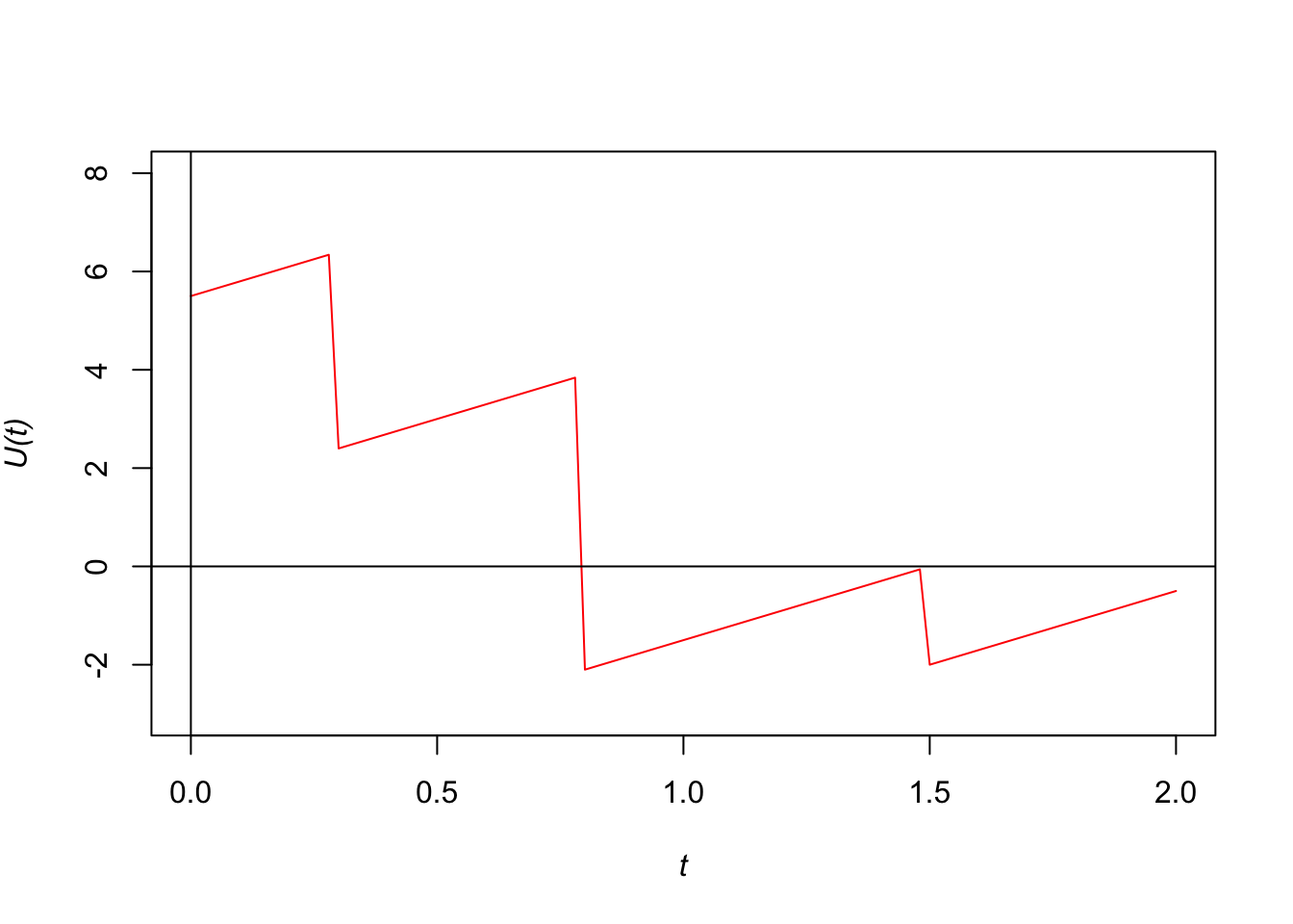
Figure 6.1: The surplus process befor reinsurance arrangment.
Ruin occurs at time 0.8 when ruin is checked continuously.
Similarly, we have \(U(1) = -1.5\) and \(U(2) = -0.5\). Therefore, ruin occurs at time 1 and 2 when ruin is checked at the end of each year.
- The insurer’s net premium income is 2 per year. The insurer’s cash flow or surplus process is now given by \[\begin{equation} U_I(t) = u + (c - c_r)t - S_I(t) = 5.5 + (3 - 1) t - S_I(t), \end{equation}\] where \(c_r\) is the reinsurance premium rate. Claims that are involved the insurer after are
| Time (year) | 0.3 | 0.8 | 1.5 |
|---|---|---|---|
| Amount | 3.5 | 3.5 | 2 |
The following table summarises the values of the surplus function at the time when claims occurs.
| Time | Surplus (before claim) | Surplus (after claim) |
|---|---|---|
| 0 | 5.5 | 5.5 |
| 0.3 | 6.1 | 2.6 |
| 0.8 | 3.6 | 0.1 |
| 1.5 | 1.5 | -0.5 |
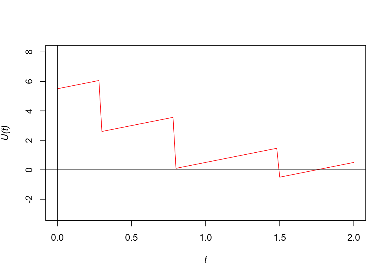
Figure 6.2: The surplus process under a reinsurance arrangement.
Under the reinsurance arrangement,
Ruin occurs at time 1.5 when ruin is checked continuously.
Similarly, we have \(U(1) = 0.5\) and \(U(2) = 0.5\). Therefore, ruin does not occur when ruin is checked at the end of each year.
- According to the property of the aggregate claims process \(S(t)\), the aggregate claims in the \(n\)th year, for \(n = 1,2, \ldots\) are \(S(n) - S(n-1) \sim \mathcal{CP}(\lambda, F_X(x))\), all of them have the same compound Poisson distribution with the same parameters. Hence, the premium rate per year will be constant which can be obtained from \[c = (1 + \theta)\text{E}[S],\] where \(\theta = 0.1\). Note that \(\text{E}[S] = \lambda \text{E}[X] = 0.1 \cdot 59.75 = 5.975\) and hence \(c = 6.5725.\)
The surplus at time 2 is \[U(2) = u + ct - S(2) = 100 + 6.5725 \cdot 2 - S(2) = 113.145 - S(2).\] So the required probability is \[\Pr(U(2) < 0) = \Pr(S(2) > 113.145) = 1- \Pr(S(2) \le 113.145).\] We consider all possibilities that \(S(2) \le s0\). According to the information from the following table,
| Number of claims | Amount of claims |
|---|---|
| 0 claim | 0 |
| 1 claim | 50 or 75 |
| 2 claims | 100 = 50 + 50 |
It follows that \[ \begin{aligned} \Pr(S(2) \le 113.145) &= \Pr(N(2) = 0) + \Pr(N(2) = 1 \text{ and } X_1 = 50) \\ &+ \Pr(N(2) = 1 \text{ and } X_1 = 70) + \Pr(N(2) = 2 \text{ and } X_1 = X_2 = 50).\\ \end{aligned} \] Note that \[ \begin{aligned} \Pr(N(2) = 0) &= 0.8187308 \\ \Pr(N(2) = 1 \text{ and } X_1 = 50) &= \Pr(N(2) = 1) \cdot \Pr(X_1 = 50) = (0.1637462)(0.7) = 0.1146223 \\ \Pr(N(2) = 1 \text{ and } X_1 = 75) &= \Pr(N(2) = 1) \cdot \Pr(X_1 = 75) = (0.1637462)(0.25) = 0.0409365 \\ \Pr(N(2) = 2 \text{ and } X_1 = X_2 = 50) &= \Pr(N(2) = 2) \cdot \Pr(X_1 = 50) \cdot \Pr(X_2 = 50)= (0.0163746)(0.7)^2 = 0.0080236 \end{aligned} \] Therefore, $(S(2) ) = 0.9823132 and \[\Pr(U(2) < 0) = \Pr(S(2) > 113.145) = 1- \Pr(S(2) \le 113.145) = 1 - 0.9823132 = 0.0176868.\]
Ruin will occur in the first year if and only if a claim (of any amount) occurs. Therefore, \[\psi(0.3,1) = 1 - \Pr(N(1) = 0) = 0.0951626.\]
In a two year time interval, ruin will not occur if and only if there are no claims before time 1.75 years (at which point the insurer’s premium income plus initial surplus is equal to 1) AND there are no claims or at most one claim of amount 1 between the time interval 1.75 to 2. \[ \begin{aligned} 1- \psi(0.3,1) &= \Pr(N(1.75) = 0) \cdot [ \Pr(N(2) - N(1.75) = 0 \text{ or } (N(2) - N(1.75) = 1 \text{ and } X_1 = 1) ] \\ &= \Pr(N(1.75) = 0) \cdot [ \Pr(N(2) - N(1.75) = 0) + \Pr(N(2) - N(1.75) = 1 \text{ and } X_1 = 1) ]. \end{aligned} \] We have \[ \begin{aligned} \Pr(N(1.75) = 0) &= 0.839457 \\ \Pr(N(2) - N(1.75) = 0) &= 0.9753099 \\ \Pr(N(2) - N(1.75) = 1 \text{ and } X_1 = 1) &= \Pr(N(2) - N(1.75) = 1) \cdot \Pr(X_1 = 1) = (0.0243827) \cdot (0.7) = 0.0170679. \end{aligned} \]
Therefore, \[1- \psi(0.3,1) = 0.839457\cdot (0.9753099 + 0.0170679) = 0.8330585, \] and \[\psi(0.3,1) = 0.1669415.\]
6.14 Tutorial 8
The table below gives the payments (in 000s THB) in cumulative form in successive development years in respect of a motor insurance portfolio. All claims are assumed to be fully settled by the end of development year 4. Use the chain ladder method to estimate the amount the insurer will pay in the calendar years \(2018, 2019, 2020 ,2021\).
Development year 0 1 2 3 4 2013 750 768 844 929 1072 Accident 2014 820 876 946 1041 Year 2015 960 997 1096 2016 1040 1087 2017 1180 The table below shows the claims payments (in 000s THB) in cumulative form for a portfolio of insurance policies. All claims are assumed to be fully settled by the end of development year 4 and the payments are made at the middle of each calendar year. The past rates of inflation over the 12 months up to the middle of the given year are as follows:
2014 5% 2015 6% 2016 7% 2017 5% The future rate of inflation from mid-2017 is assumed to be 10% per year.
Development year 0 1 2 3 4 2013 880 988 1046 1065 1262 Accident 2014 940 1034 1091 1095 Year 2015 1060 1161 1229 2016 1120 1221 2017 1240 Use the inflation-adjusted chain ladder method to calculate the outstanding claims payments in future years.
Using an interest rate of 7% per year, calculate the outstanding claims reserve the insurer should have hold on 1 January 2018.
The table below shows the cumulative claims payments and the cumulative number of claims (amounts appear above claim numbers) for a portfolio of insurance policies. All claims are assumed to be fully settled by the end of development year 5 and that the effects of claims-cost inflation have been removed from these data. Use the average cost per claim method to estimate the outstanding claims reserve which should be held at the end of 2017.
Development year 0 1 2 3 4 5 2012 2800 2954 3005 3275 3624 3895 420 440 453 493 551 591 2013 3200 3379 3449 3760 4184 460 478 490 533 591 Accident 2014 3800 4004 4078 4454 Year 500 525 531 580 2015 4520 4749 4842 520 549 558 2016 5340 5587 560 589 2017 5840 570 The table below shows the cumulative claims payments and the premium income \(P\) for a portfolio of insurance policies. All claims are assumed to be fully settled by the end of development year 4 and that the effects of claims-cost inflation have been removed from these data. Use the Bornhuetter-Ferguson method to estimate the total reserve required to meet the outstanding claims. You may assume that the ultimate loss ratio for accident years 2014-2017 will be 95%.
Development year 0 1 2 3 4 \(P\) 2013 3597 4226 4547 4807 4989 5937 Accident 2014 4174 4697 5317 5497 6122 Year 2015 4578 5082 5753 6221 2016 4634 5343 6365 2017 5203 6510
6.16 Tutorial 9
(Taken from Gray and Pitts) Suppose the number of claims which arise in a year on a group of policies is modelled as \(X|\lambda \sim Poisson(\lambda)\) and that we observe a total of 14 claims over a six year period. Suppose also we adopt a \(\mathcal{G}(6, 3)\) distribution as a prior distribution for \(\lambda\).
State the maximum likelihood estimate of \(\lambda\) and the prior mean.
State the posterior distribution of \(\lambda\), find the mode of this distribution, and hence state the Bayesian estimate of \(\lambda\) under all or nothing loss.
Note that if \(Y \sim \mathcal{G}(\alpha,\beta)\) and \(2\alpha\) is an integer, then \(2\beta Y \sim \mathcal{G}(\alpha,1/2)\); that is \(2\beta Y \sim \chi^2\) with \(2 \alpha\) degrees of freedom.
Using this fact, find the Bayesian estimate of \(\lambda\) under absolute error loss.
Find an equal-tailed 95% Bayesian interval estimate of \(\lambda\), that is an interval \((\lambda_L, \lambda_U)\), such that \(Pr( \lambda > \lambda_U | \underline{x}) = Pr( \lambda < \lambda_L | \underline{x}) = 0.025\).
Find the credibility estimate (the Bayesian estimate under squared-error loss) of \(\lambda\).
Recall that the data \(x_1, x_2, \ldots, x_n\) are available on \(X | \lambda\). Suppose we observe \(\sum x_i = 13\) when \(n = 50\). Based on the Poisson\(-\)Gamma model, the number of claims which arise in a year on a group of policies is modelled as \(X|\lambda \sim Poisson(\lambda)\) and the prior distribution on the claim rate \(\lambda\) is a \(\mathcal{G}(\alpha,\beta)\) distribution.
Calculate the value of the maximum likelihood estimate of \(\lambda\)
Calculate the values of prior means and the prior variance in two cases (i) the prior is \(\mathcal{G}(6,30)\) and (ii) the prior is \(\mathcal{G}(2,10)\). Comment on the results.
For those two prior distributions, calculate the posterior mean of \(\lambda\) given such data.
Suppose the annual claims which arise under a risk, \(X\), in units of 1000THB, as \(X | \theta \sim \mathcal{N}(\theta,0.36)\). From experience with other business, an insurer adopt a \(\mathcal{N}(2, 0.04)\) prior for \(\theta\). The insurer observe claim amounts for the past seven years : \(2369, 2341, 2284, 2347, 2332, 2300, 2267\) THB. Using the normal\(-\)normal model:
Find the credibility factor and the credibility premium for the risk.
Find an equal-tailed 95% Bayesian interval estimate of \(\theta\).
Consider a collective of five separate risks from portfolios of general insurance policies, each of which has been in existence for at least ten years. The mean and variance of the aggregate claims adjusted for inflation over the past ten years are given in the table. Use EBCT Model 1 to calculate the credibility premiums for all five risks.
Risk Within risk mean Within risk variance 1 138 259 2 98 179 3 120 239 4 104 168 5 119 185 Consider the aggregate claims in five successive years from comparable insurance policies (in units of 1000 THB).
\[TableRisks\]
Year \(j\) 1 2 3 4 5 Risk \(i\) 1 68 65 77 76 74 2 54 59 56 50 62 3 81 95 83 82 89 4 64 70 77 66 73 Use the EBCT Model 1 to calculate the credibility premium for each risk \(i\).
Explain why the credibility premiums depend almost entirely on the means for the individual risks.
6.17 Solutions to Tutorial 9
- Based on the lecture note, the data consist of \(n\) observations \(x_1, x_2, \ldots, x_n\) of random variables \(X_1, \ldots , X_n\), where, given \(\lambda\), the \(X_i\) are iid Poisson random variables with parameter \(\lambda\) for \(i = 1,\ldots,n\).
The likelihood is given by \[ f(\underline{x}|\lambda) = \Pi_{i=1}^n \frac{e^{-\lambda} \lambda^{x_i}}{x_i!} \propto e^{-n\lambda} \lambda^{\sum x_i}. \] Therefore, the data-based estimator of \(\lambda\) based on the maximum likelihood estimator is \[\hat{\lambda} = \frac{\sum_i x_i}{n} = \frac{14}{6} = 2.3333333.\]
Without any data from the risk, a reasonable estimate value of \(\lambda\) is the mean of the prior distribution with both parameters known and with density function \[ f(\lambda) = \frac{\beta^\alpha}{\Gamma(\alpha)} \lambda^{\alpha -1} e^{-\beta\lambda}, \quad \alpha >0, \, \beta > 0, \, \lambda > 0.\] It follows that the estimate of \(\lambda\) using the prior mean is \[ \tilde{\lambda} = \frac{\alpha}{\beta} = \frac{6}{3} = 2.\]
- The posterior density is proportional to
\[ \begin{aligned} f(\lambda| \underline{x}) &\propto (\lambda^{\alpha -1} e^{-\beta\lambda}) (e^{-n\lambda} \lambda^{\sum x_i}) \\ &= \lambda^{\alpha + \sum x_i -1} e^{-(\beta + n) \lambda} \end{aligned} \] This is the functional part of a gamma density. The posterior distribution is \[ \lambda | \underline{x} \sim \mathcal{G}(\alpha + \sum x_i, \beta + n) = \mathcal{G}(20, 9).\]
The Bayesian estimator of \(\lambda\) under the all or nothing loss is the mode of the distribution, which is given by \[\frac{19}{9} = 2.1111111.\]
Under absolute error loss, the median of\(\mathcal{G}(20, 9)\) can be found by using the following R syntax \[\text{qgamma}(0.5, \text{shape}= 20, \text{rate}=9) = 2.1852969\] Moreover, we can get \[\lambda_L = \text{qgamma}(0.025, \text{shape}= 20, \text{rate}=9) = 1.3573911\] and \[\lambda_U = \text{qgamma}(0.975, \text{shape}= 20, \text{rate}=9) = 3.2967615.\]
The credibility estimate (i.e. the mean of \(\mathcal{G}(20, 9)\)) is
\[ \begin{aligned} \lambda^* &= \frac{\alpha + \sum x_i}{ \beta + n} = \frac{20}{9} = 2.2222222. \end{aligned}, \] where \(Z = n/(n+\beta)\). This can be expressed in the form of a credibility estimate. \end{enumerate}
- From the Poisson-Gamma model,
- Therefore, the data-based estimator of \(\lambda\) based on the maximum likelihood estimator is \[\hat{\lambda} = \frac{\sum_i x_i}{n} = \frac{13}{50} = 0.26.\]
- For \(\lambda \sim \mathcal{G}(\alpha,\beta)\), we have \[\text{E}[\lambda] = \frac{\alpha}{\beta} \text{ and } \text{Var}[\lambda] = \frac{\alpha}{\beta^2}.\]
For \(\mathcal{G}(6, 30)\), the prior mean and prior variance are 0.2 and 0.0066667, respectively.
For \(\mathcal{G}(2, 10)\), the prior mean and prior variance are 0.2 and 0.02, respectively.
The variance of the prior distributions are 0.0066667 and 0.02 in (i) and (ii), respectively. There is more uncertainty in the prior distribution of (ii) which leads to the prior mean getting lower weight. Therefore, \(Z\) should be larger in (ii).
- The posterior mean of \(\lambda\) (also denoted by CP) is
\[ \begin{aligned} \text{CP} &= (Z) \left( \frac{\sum x_i}{n} \right) +(1-Z) \left( \frac{\alpha}{\beta} \right) \end{aligned}, \] where \(Z = n/(n+\beta)\). This can be expressed in the form of a credibility estimate.
In this case, \(Z = \frac{50}{50 + 30} = 0.625\) and \(\text{CP} = 0.2375\).
In this case, \(Z = \frac{50}{50 + 10} = 0.8333333\) and \(\text{CP} = 0.25\).
We have \(\sum_{i=1}^7 x_i = `r `sumx`\). The credibility factor \(Z\) is given by \[ Z = \frac{n}{n + \frac{\sigma^2}{{\sigma_0^2}}} = 0.4375.\] The credibility premium is \[\text{CP} = Z\cdot\frac{\sum x_i}{n} + (1-Z)\cdot \mu_0 = 2140.\]
The posterior probability distribution function is \(\mathcal{N}(\mu^*,\sigma^{*2})\), where (in unit of 1000) \[\mu^* = 2.14 \text{ and } \sigma^{*2} = \frac{\sigma_0^2\sigma^2}{n\sigma_0^2 + \sigma^2} = 0.0225.\] Therefore, using the following R commands, \[\mu_L = \text{qnorm}(0.025,2.14,\sqrt{0.0225}) = 1.8460054,\] and \[\mu_U = \text{qnorm}(0.975,2.14,\sqrt{0.0225}) = 2.4339946.\]
Not in the Final Examination.
Not in the Final Examination.