Chapter 2 Loss distributions
2.1 Introduction
The main objective of the course is to provide methods for analysing insurance data leading to decisions with an emphasis in an insurance context.
2.1.1 The importance of insurance or the benefits of insurance for society
Let us begin with the importance of insurance or the benefits of insurance for society.
The insurer protects the wealth of society through a variety of insurance plans. Life insurance provides protection against loss of human wealth. General insurance protects property from damage by fire, theft, accidents, earthquakes, etc. Consequently, both general insurance and life insurance provide security to maintain financial and business conditions.
The insurance policy is a contract between the insurer and the policyholder, which sets out the claims that the insurer is legally obliged to pay. The insurer guarantees compensation for losses caused by risks covered by the insurance policy, called the insurance claim in return for an initial payment, called the premium.
2.1.2 The types of insurance
Families and organisations that do not want to bear their own risks can choose from a variety of insurance policies.The following questions can be asked about an insurance policy (Click here for more details):
the nature of insurance is who buys it: Is it a personal, group or commercial?
the nature of insurance is the type of risk being covered: Is it a life/health insurance policy or a property/casualty policy?
the nature of insurance is by the duration of an insurance contract, known as the term: Is it a short-term or a long-term contract?
Is it issued by a private insurer or a government agency?
Was it taken out voluntarily or involuntarily?
Notes
The amount of benefits provided by life insurance policies is often specified in the policies. In contrast, most non-life insurance policies provide compensation for insured losses that were not known prior to the event (usually the compensation amounts are limited).
The time value of money is important in a life insurance contract that runs over a long period of time. In a non-life contract, the random amount of compensation takes priority.
2.1.3 Insurance Operations and Data Analytics
The ultimate goal is to use insurance data as a basis for decision-making. Throughout the course, we will learn more about techniques for analysing and extrapolating data. To begin with, we will describe five key operational areas of insurance companies and highlight the role of data and analytics in each operational area.
Initiate insurance: The company decides at this stage whether or not to accept a risk (the underwriting step) and then determines the appropriate premium (or rate). The basics of insurance analysis are found in ratemaking, where analysts try to find the appropriate price for the appropriate risk.
Renewal of insurance: Many policies, especially in general insurance, are only valid for a few months or a year. The insurer has the option of refusing cover and changing the premium, even though it assumes that such contracts would be renewed. The purpose of this phase of policy renewal, where analytics are also used, is to retain profitable customers.
Claims management: Analytics have been used for years to (1) identify claims. and prevent claims fraud, (2) control claims costs, including identifying the right type of support to cover the costs associated with claims handling, and (3) capture additional layers for reinsurance and retention.
Reserves for losses: Management obtains an accurate estimate of future responsibilities using analytical techniques, and the uncertainty of these predictions is quantified.
Capital allocation and solvency: Among the important analytical operations is the choice of the amount of capital required and its allocation to the various investments. Companies need to be aware of their capital requirements in order to have sufficient cash flow to meet their obligations when they are likely to occur (solvency). This is an important concern not only for management, but also for clients, shareholders, regulators and the public.
2.2 Loss Distributions
The aim of the course is to provide a fundamental basis which applies mainly in general insurance. General insurance companies’ products are short-term policies that can be purchased for a short period of time. Examples of insurance products are
motor insurance;
home insurance;
health insurance; and
travel insurance.
In case of an occurrence of an insured event, two important components of financial losses which are of importance for management of an insurance company are
the number of claims; and
the amounts of those claims.
Mathematical and statistical techniques used to model these sources of uncertainty will be discussed. This will enable insurance companies to
calculate premium rates to charge policy holders; and
decide how much reserve should be set aside for the future payment of incurred claims.
In the chapter, statistical distributions and their properties which are suitable for modelling claim sizes are reviewed. These distribution are also known as loss distributions. In practice, the shape of loss distributions are positive skew with a long right tail. The main features of loss distributions include:
having a few small claims;
rising to a peak;
tailing off gradually with a few very large claims.
2.3 Exponential Distribution
A random variable \(X\) has an exponential distribution with a parameter \(\lambda > 0\), denoted by \(X \sim \text{Exp}(\lambda)\) if its probability density function is given by \[f_X(x) = \lambda e^{-\lambda x}, \quad x > 0.\]
Example 2.1 Let \(X \sim \text{Exp}(\lambda)\) and \(0 < a < b\).
Find the distribution \(F_X(x)\).
Express \(P(a < X < B)\) in terms of \(f_X(x)\) and \(F_X(x)\).
Show that the moment generating function of \(X\) is \[M_X(t) = \left(1 - \frac{t}{\lambda}\right)^{-1}, \quad t < \lambda.\]
Derive the \(r\)-th moment about the origin \(\mathrm{E}[X^r].\)
Derive the coefficient of skewness for \(X\).
Simulate a random sample of size n = 200 from \(X \sim \text{Exp}(0.5)\) using the command
sample = rexp(n, rate = lambda)where \(n\) and \(\lambda\) are the chosen parameter values.Plot a histogram of the random sample using the command
hist(sample)(use help for available options forhistfunction in R).
Solution: The code for questions 6 and 7 is given below. The histogram can be generated from the code below.
# set.seed is used so that random number generated from different simulations are the same.
# The number 5353 can be set arbitrarily.
set.seed(5353)

nsample <- 200
data_exp <- rexp(nsample, rate = 0.5)

dataset <- data_exp
hist(dataset, breaks=100,probability = TRUE, xlab = "claim sizes"
     , ylab = "density", main = paste("Histogram of claim sizes" ))

hist(dataset, breaks=100, xlab = "claim sizes"
     , ylab = "count", main = paste("Histogram of claim sizes" ))
Copy and paste the code above and run it.
Notes
The exponential distribution can used to model the inter-arrival time of an event.
The exponential distribution has an important property called lack of memory: if \(X \sim \text{Exp}(\lambda)\), then the random variable \(X-w\) conditional on \(X > w\) has the same distribution as \(X\), i.e. \[X \sim \text{Exp}(\lambda)\Rightarrow X - w | X > w \sim \text{Exp}(\lambda).\]
We can use R to plot the probability density functions (pdf) of exponential distributions with various parameters \(\lambda\), which are shown in Figure 2.1. Here we use scale_colour_manual to override defaults with scales package (see cheat sheet for details).
library(ggplot2)
ggplot(data.frame(x=c(0,10)), aes(x=x)) +
  labs(y="Probability density", x = "x") +
  ggtitle("Exponential distributions") +
  theme(plot.title = element_text(hjust = 0.5)) +
  stat_function(fun=dexp,geom ="line", args = (mean=0.5), aes(colour = "0.5")) +
  stat_function(fun=dexp,geom ="line", args = (mean=1), aes(colour = "1")) +
  stat_function(fun=dexp,geom ="line", args = (mean=1.5), aes(colour = "1.5")) +
  stat_function(fun=dexp,geom ="line", args = (mean=2), aes(colour = "2")) +
  scale_colour_manual(expression(paste(lambda, " = ")), values = c("red", "blue", "green", "orange"))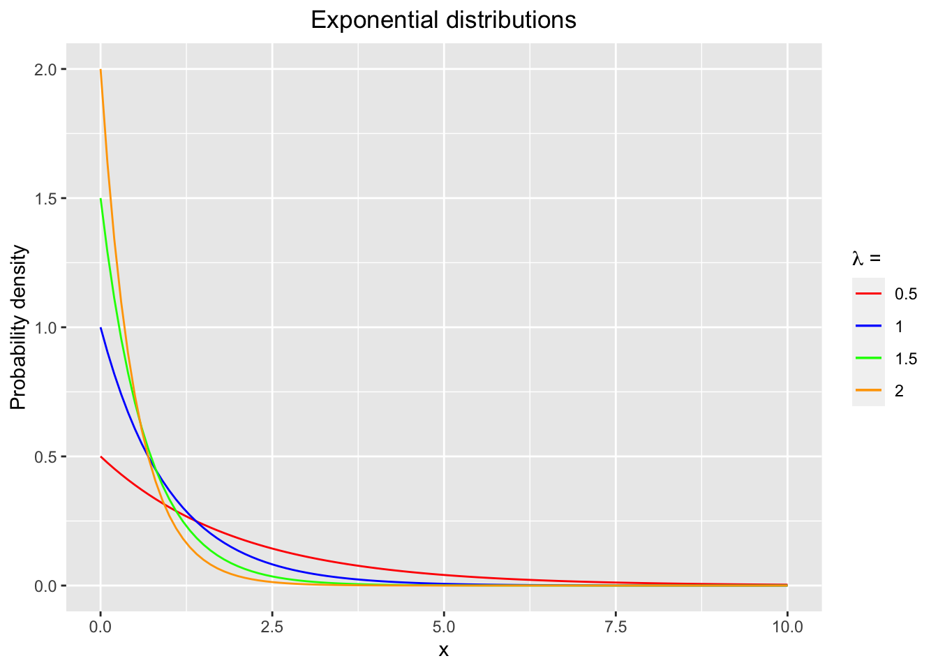
Figure 2.1: The probability density functions (pdf) of exponential distributions with various parameters lambda.
2.4 Gamma distribution
A random variable \(X\) has a gamma distribution with parameters \(\alpha > 0\) and \(\lambda > 0\), denoted by \(X \sim \mathcal{G}(\alpha, \lambda)\) or \(X \sim \text{gamma}(\alpha, \lambda)\) if its probability density function is given by \[f_X(x) = \frac{\lambda^\alpha}{\Gamma(\alpha)} x^{\alpha -1} e^{-\lambda x}, \quad x > 0.\] The symbol \(\Gamma\) denotes the gamma function, which is defined as \[\Gamma(\alpha) = \int_{0}^\infty x^{\alpha - 1} e^{-x} \mathop{}\!dx, \quad \text{for } \alpha > 0.\] It follows that \(\Gamma(\alpha + 1) = \alpha \Gamma(\alpha)\) and that for a positive integer \(n\), \(\Gamma(n) = (n-1)!\).
The properties of the gamma distribution are summarised.
The mean and variance of \(X\) are \[\mathrm{E}[X] = \frac{\alpha}{\lambda} \text{ and } \mathrm{Var}[X] =\frac{\alpha}{\lambda^2}\]
The \(r\)-th moment about the origin is \[\mathrm{E}[X^r] = \frac{1}{\lambda^r} \frac{\Gamma(\alpha + r)}{\Gamma(\alpha )}, \quad r > 0.\]
The moment generating function (mgf) of \(X\) is \[M_X(t) = \left(1 - \frac{t}{\lambda}\right)^{-\alpha}, \quad t < \lambda.\]
The coefficient of skewness is \[\frac{2}{\sqrt{\alpha}}.\]
Notes 1. The exponential function is a special case of the gamma distribution, i.e. \(\text{Exp}(\lambda)= \mathcal{G}(1,\lambda)\)
If \(\alpha\) is a positive integer, the sum of \(\alpha\) independent, identically distributed as \(\text{Exp}(\lambda)\), is \(\mathcal{G}(\alpha, \lambda)\).
If \(X_1, X_2, \ldots, X_n\) are independent, identically distributed, each with a \(\mathcal{G}(\alpha, \lambda)\) distribution, then \[\sum_{i = 1}^n X_i \sim \mathcal{G}(n\alpha, \lambda).\]
The exponential and gamma distributions are not fat-tailed, and may not provide a good fit to claim amounts.
Example 2.2 Using the moment generating function of a gamma distribution, show that the sum of independent gamma random variables with the same scale parameter \(\lambda\), \(X \sim \mathcal{G}(\alpha_1, \lambda)\) and \(Y \sim \mathcal{G}(\alpha_2, \lambda)\), is \(S = X+ Y \sim \mathcal{G}(\alpha_1 + \alpha_2, \lambda).\)
Solution: Because \(X\) and \(Y\) are independent, \[\begin{aligned} M_S(t) &= M_{X+Y}(t) = M_X(t) \cdot M_Y(t)\\ &= (1 - \frac{t}{\lambda})^{-\alpha_1} \cdot (1 - \frac{t}{\lambda})^{-\alpha_2} \\ &= (1 - \frac{t}{\lambda})^{-(\alpha_1 + \alpha_2)}. \end{aligned}\] Hence \(S = X + Y \sim \mathcal{G}(\alpha_1 + \alpha_2, \lambda).\)
The probability density functions (pdf) of gamma distributions with various shape parameters \(\alpha\) and rate parameter \(\lambda\) = 1 are shown in Figure 2.2.
ggplot(data.frame(x=c(0,20)), aes(x=x)) +
  labs(y="Probability density", x = "x") +
  ggtitle("Gamma distribution")  +
  theme(plot.title = element_text(hjust = 0.5)) +
  stat_function(fun=dgamma, args=list(shape=2, rate=1), aes(colour = "2")) +
  stat_function(fun=dgamma, args=list(shape=6, rate=1) , aes(colour = "6")) +
  scale_colour_manual(expression(paste(lambda, " = 1 and ", alpha ," = ")), values = c("red", "blue"))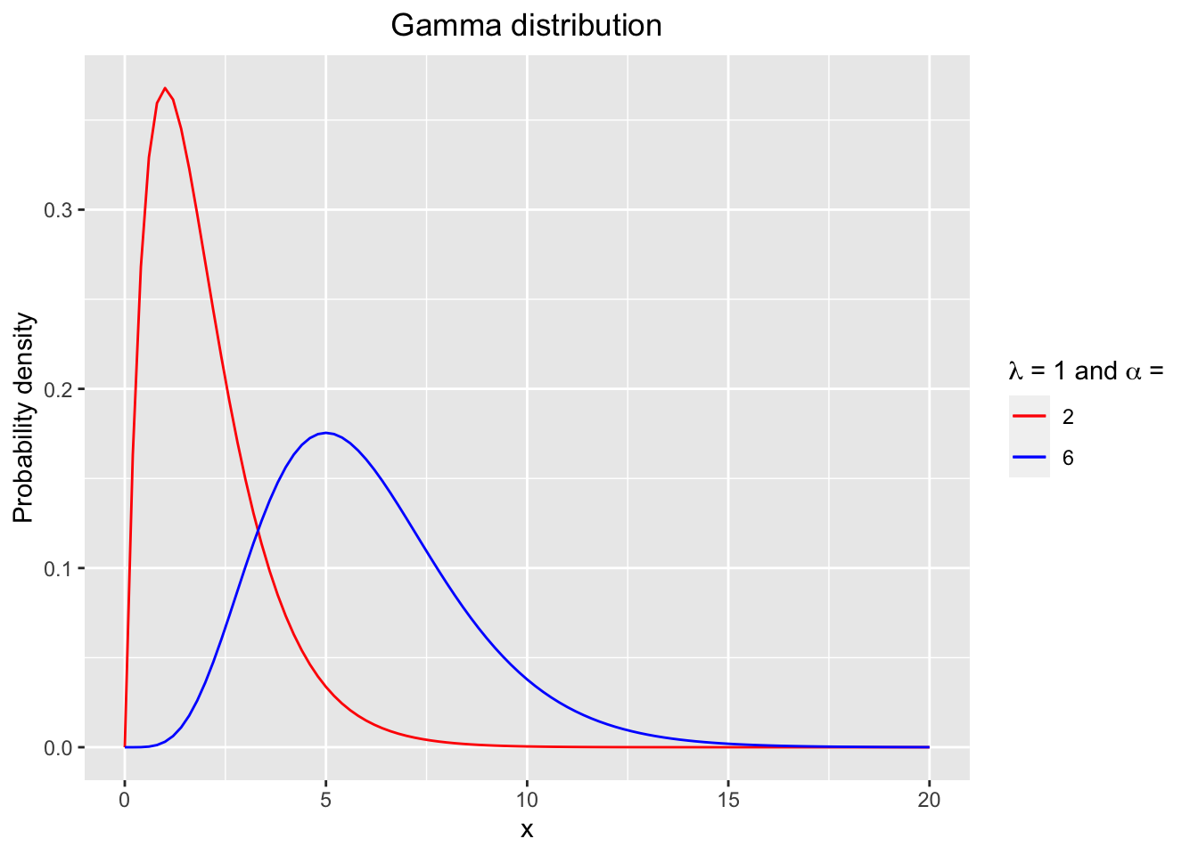
Figure 2.2: The probability density functions (pdf) of gamma distributions with various shape alpha and rate parameter lambda = 1.
2.5 Lognormal distribution
A random variable \(X\) has a lognormal distribution with parameters \(\mu\) and \(\sigma^2\), denoted by \(X \sim \mathcal{LN}(\mu, \sigma^2)\) if its probability density function is given by \[f_X(x) = \frac{1}{\sigma x \sqrt{2 \pi}} \exp\left(-\frac{1}{2} \left( \frac{\log(x) - \mu}{\sigma} \right)^2 \right) , \quad x > 0.\]
The following relation holds: \[X \sim \mathcal{LN}(\mu, \sigma^2)\Leftrightarrow Y = \log X \sim \mathcal{N}(\mu, \sigma^2).\]
The properties of the lognormal distribution are summarised.
The mean and variance of \(X\) are \[\mathrm{E}[X] = \exp\left(\mu + \frac{1}{2} \sigma^2 \right) \text{ and } \mathrm{Var}[X] =\exp\left(2\mu + \sigma^2 \right) (\exp(\sigma^2) - 1).\]
The \(r\)-th moment about the origin is \[\mathrm{E}[X^r] =\exp\left(r\mu + \frac{1}{2}r^2 \sigma^2 \right).\]
The moment generating function (mgf) of \(X\) is not finite for any positive value of \(t\).
The coefficient of skewness is \[(\exp(\sigma^2) + 2) \left(\exp(\sigma^2) -1 \right)^{1/2} .\]
The probability density functions (pdf) of gamma distributions with various shape parameters \(\alpha\) and rate parameter \(\lambda = 1\) is shown in Figure 2.3.
ggplot(data.frame(x=c(0,10)), aes(x=x)) +
  labs(y="Probability density", x = "x") +
  ggtitle("lognormal distribution")  +
  theme(plot.title = element_text(hjust = 0.5)) +
  stat_function(fun=dlnorm, args = list(meanlog = 0, sdlog = 0.25), aes(colour = "0.25")) +
  stat_function(fun=dlnorm, args = list(meanlog = 0, sdlog = 1), aes(colour = "1")) +
  scale_colour_manual(expression(paste(mu, " = 0 and ", sigma, "= ")), values = c("red", "blue"))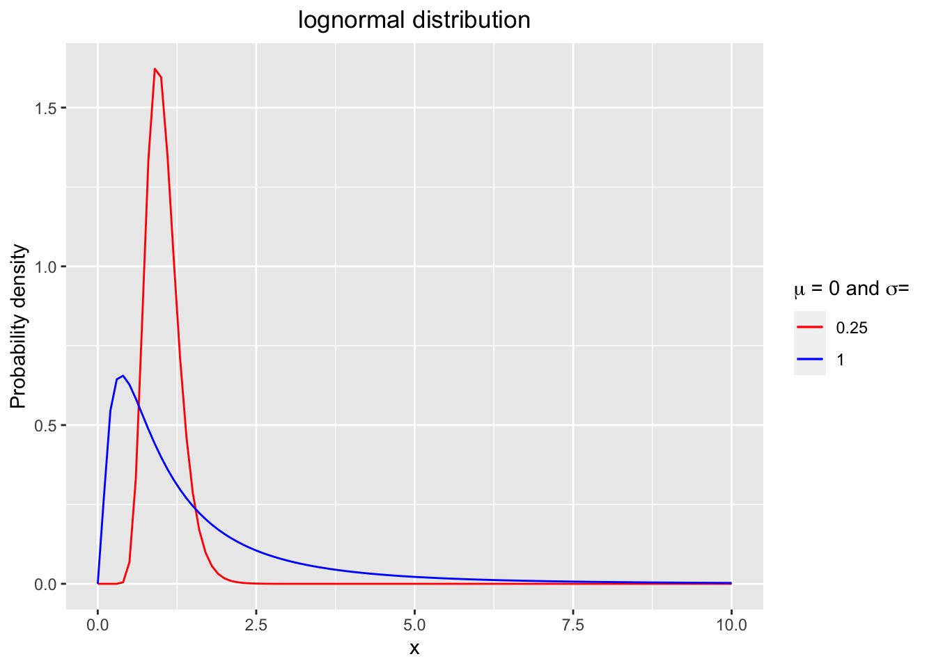
Figure 2.3: The probability density functions (pdf) of lognormal distributions with mu = 0 and sigma = 0.25 or 1.
2.6 Pareto distribution
A random variable \(X\) has a Pareto distribution with parameters \(\alpha > 0\) and \(\lambda > 0\), denoted by \(X \sim \text{Pa}(\alpha, \lambda)\) if its probability density function is given by \[f_X(x) = \frac{\alpha \lambda^\alpha}{(\lambda + x)^{\alpha + 1}}, \quad x > 0.\] The distribution function is given by \[F_X(x) = 1 - \left( \frac{\lambda}{\lambda + \alpha} \right)^\alpha, \quad x > 0.\]
The properties of the Pareto distribution are summarized.
The mean and variance of \(X\) are \[\mathrm{E}[X] = \frac{\lambda}{\alpha - 1}, \alpha > 1 \text{ and } \mathrm{Var}[X] = \frac{\alpha \lambda^2}{(\alpha - 1)^2(\alpha - 2)}, \alpha > 2.\]
The \(r\)-th moment about the origin is \[\mathrm{E}[X^r] =\frac{\Gamma(\alpha-r) \Gamma(1+ r)}{\Gamma(\alpha)} \lambda^r, \quad 0 < r < \alpha.\]
The moment generating function (mgf) of \(X\) is not finite for any positive value of \(t\).
The coefficient of skewness is \[\frac{2(\alpha + 1)}{\alpha - 3} \sqrt{\frac{\alpha-2}{\alpha}} , \quad \alpha > 3.\]
Note 1. The following conditional tail property for a Pareto distribution is useful for reinsurance calculation. Let \(X \sim \text{Pa}(\alpha, \lambda)\). Then the random variable \(X - w\) conditional on \(X > w\) has a Pareto distribution with parameters \(\alpha\) and \(\lambda + w\), i.e. \[X \sim \text{Pa}(\alpha, \lambda)\Rightarrow X - w | X > w \sim \text{Pa}(\alpha,\lambda + w).\]
The lognormal and Pareto distributions, in practice, provide a better fit to claim amounts than exponential and gamma distributions.
Other loss distribution are useful in practice including Burr, Weibull and loggamma distributions.
library(actuar)
ggplot(data.frame(x=c(0,60)), aes(x=x)) +
  labs(y="Probability density", x = "x") +
  ggtitle("Pareto distribution")  +
  theme(plot.title = element_text(hjust = 0.5)) +
  stat_function(fun=dpareto, args=list(shape=3, scale=20), aes(colour = "alpha = 3, lambda = 20")) +
  stat_function(fun=dpareto, args=list(shape=6, scale=50), aes(colour = "alpha = 6, lambda = 50")) +
scale_colour_manual("Parameters", values = c("red", "blue"), labels = c(expression(paste(alpha, " = 3 and ", lambda, "= 20")), expression(paste(alpha, " = 6 and ", lambda, "= 50")))) 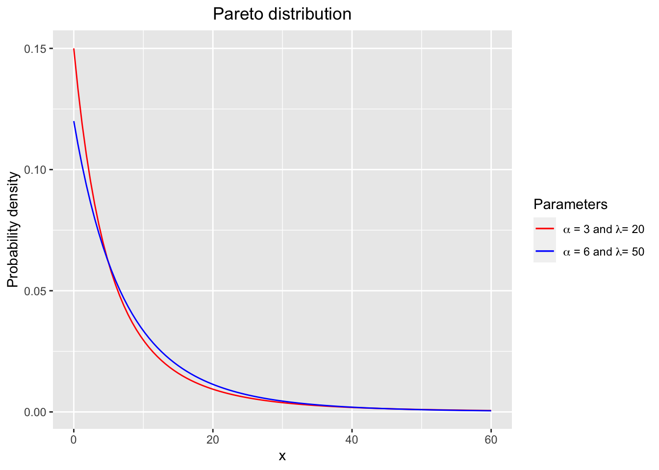
Figure 2.4: The probability density functions (pdf) of Pareto distributions with various shape alpha and rate parameter lambda = 1.
Example 2.3 Consider a data set consisting of 200 claim amounts in one year from a general insurance portfolio.
Calculate the sample mean and sample standard deviation.
Use the method of moments to fit these data with both exponential and gamma distributions.
Calculate the boundaries for groups or bins so that the expected number of claims in each bin is 20 under the fitted exponential distribution.
Count the values of the observed claim amounts in each bin.
With these bin boundaries, find the expected number of claims when the data are fitted with the gamma, lognormal and Pareto distributions.
Plot a histogram for the data set along with fitted exponential distribution and fitted gamma distribution. In addition, plot another histogram for the data set along with fitted lognormal and fitted Pareto distribution.
Comment on the goodness of fit of the fitted distributions.
Solution: 1. Given that \(\sum_{i=1}^n x_i = 206046.4\) and \(\sum_{i=1}^n x_i^2 = 1,472,400,135\), we have \[\bar{x} = \frac{\sum_{i=1}^n x_i}{n} = \frac{206046.4}{200} = 1030.232.\] The sample variance and standard deviation are \[s^2 = \frac{1}{n-1} \left( \sum_{i=1}^n x_i^2 - \frac{(\sum_{i=1}^n x_i)^2}{n} \right) = 6332284,\] and \[s = 2516.403.\]
We calculate estimates of unknown parameters of both exponential and gamma distributions by the method of moments. We simply match the mean and central moments, i.e. matching \(\mathrm{E}[X]\) to the sample mean \(\bar{x}\) and \(\mathrm{Var}[X]\) to the sample variance.
The MME (moment matching estimation) of the required distributions are as follows:
the MME of \(\lambda\) for an \(\text{Exp}(\lambda)\) distribution is the reciprocal of the sample mean, \[\tilde{\lambda} = \frac{1}{\bar{x}} = 0.000971.\]
the MMEs of \(\alpha\) and \(\lambda\) for a \(\mathcal{G}(\alpha, \lambda)\) distribution are \[\begin{aligned} \tilde{\alpha} &= \left(\frac{\bar{x}}{s}\right)^2 = 0.167614, \\ \tilde{\lambda} &= \frac{\tilde{\alpha}}{\bar{x}} = 0.000163.\end{aligned}\]
the MMEs of \(\mu\) and \(\sigma\) for a \(\mathcal{LN}(\mu, \sigma^2)\) distribution are \[\begin{aligned} \tilde{\sigma} &= \sqrt{ \ln \left( \frac{s^2}{\bar{x}^2} + 1 \right) } = 1.393218, \\ \tilde{\mu} &= \ln(\bar{x}) - \frac{\tilde{\sigma}^2 }{2} = 5.967012.\end{aligned}\]
the MMEs of \(\alpha\) and \(\lambda\) for a \(\text{Pa}(\alpha, \lambda)\) distribution are \[\begin{aligned} \tilde{\alpha} &= \displaystyle{ 2 \left( \frac{s^2}{\bar{x}^2} \right) \frac{1}{(\frac{s^2}{\bar{x}^2} - 1)} } = 2.402731,\\ \tilde{\lambda} &= \bar{x} (\tilde{\alpha} - 1) = 1445.138.\end{aligned}\]
The upper boundaries for the 10 groups or bins so that the expected number of claims in each bin is 20 under the fitted exponential distribution are determined by \[\Pr(X \le \text{upbd}_j) = \frac{j}{10}, \quad j = 1,2,3, \ldots, 9.\] With \(\tilde{\lambda}\) from the MME for an \(\text{Exp}(\lambda)\) from the previous, \[\Pr(X \le x) = 1 - \exp(-\tilde{\lambda} x).\] We obtain \[\text{upbd}_j = -\frac{1}{\tilde{\lambda}} \ln\left( 1 - \frac{j}{10}\right).\] The results are given in Table 2.1.
The following table shows frequency distributions for observed and fitted claims sizes for exponential, gamma, and also lognormal and Pareto fits.
| Range | Observation | Exp | Gamma | Lognormal | Pareto |
|---|---|---|---|---|---|
| (0,109] | 60 | 20 | 109.4 | 36 | 31.9 |
| (109,230] | 31 | 20 | 14.3 | 34.4 | 27.8 |
| (230,367] | 25 | 20 | 9.7 | 26 | 24.2 |
| (367,526] | 17 | 20 | 7.8 | 20.5 | 21.2 |
| (526,714] | 14 | 20 | 6.8 | 16.6 | 18.6 |
| (714,944] | 13 | 20 | 6.3 | 13.9 | 16.4 |
| (944,1240] | 6 | 20 | 6.2 | 11.9 | 14.6 |
| (1240,1658] | 7 | 20 | 6.5 | 10.8 | 13.2 |
| (1658,2372] | 10 | 20 | 7.7 | 10.4 | 12.5 |
| (2372,\(\infty\)) | 17 | 20 | 25.4 | 19.5 | 19.4 |
Let \(X\) be the claim size.
The expected number of claims for the fitted exponential distribution in the range \((a,b]\) is \[200 \cdot \Pr( a < X \le b) = 200( e^{-\tilde{\lambda} a} - e^{-\tilde{\lambda} b} ).\] In our case, the expected frequencies under the fitted exponential distribution are given in the third column of Table 2.1.
(Excel) The expected number of claims for the fitted gamma distribution in the range \((a,b]\) is \[200 \cdot\left( \text{GAMMADIST}\left(b, \tilde{\alpha}, \frac{1}{\tilde{\lambda}}, \text{TRUE}\right) - \text{GAMMADIST}\left(a, \tilde{\alpha}, \frac{1}{\tilde{\lambda}}, \text{TRUE}\right) \right).\] The expected frequencies under the fitted gamma distribution are given in the fourth column of Table 2.1.
(Excel) For the fitted lognormal, the expected number of claims in the range \((a,b]\) can be obtained from \[200 \cdot\left( \text{NORMDIST} \left(\frac{LN(b) - \tilde{\mu}}{\tilde{\sigma}}\right) - \text{NORMDIST}\left(\frac{LN(a) - \tilde{\mu}}{\tilde{\sigma}}\right) \right).\]
For the fitted Pareto distribution, the expected number of claims in the range \((a,b]\) can be obtained from \[200 \left[ \left(\frac{\tilde{\lambda}}{\tilde{\lambda} + a} \right)^{\tilde{\alpha}} - \left(\frac{\tilde{\lambda}}{\tilde{\lambda} + b} \right)^{\tilde{\alpha}} \right].\]
The histograms for the data set with fitted distributions are shown in Figures 2.5 and 2.6.
Comments:
The high positive skewness of the sample reflects the fact that SD is large when compared to the mean. Consequently, the exponential distribution may not fit the data well.
Five claims (2.5%) are greater than 10,000, which is one of the main features of the loss distribution.
The fit is poor for the exponential distribution, as we see that the model under-fits the data for small claims up to 367 and over-fits for large claims between 944 to 2372. The gamma fit is again poor. We see that the model over-fits for small claims between 0-109 and under-fits for claims 230 and 944.
Which one of the lognormal and Pareto distributions provides a better fit to the observed claim data?
library(stats)
library(MASS)
library(ggplot2)

xbar <- mean(dat$claims)
s <- sd(dat$claims)

# MME of alpha and lambda for Gamma distribution
alpha_tilde <- (xbar/s)^2
lambda_tilde <- alpha_tilde/xbar

ggplot(dat) + geom_histogram(aes(x = claims, y = ..density..), bins = 90 , fill = "grey", color = "black") +
  stat_function(fun=dexp, geom ="line", args = (rate = 1/mean(dat$claims)), aes(colour = "Exponential")) +
  stat_function(fun=dgamma, geom ="line", args = list(shape = alpha_tilde ,rate = lambda_tilde), aes(colour = "Gamma")) + ylim(0, 0.0015) + scale_color_discrete(name="Fitted Distributions")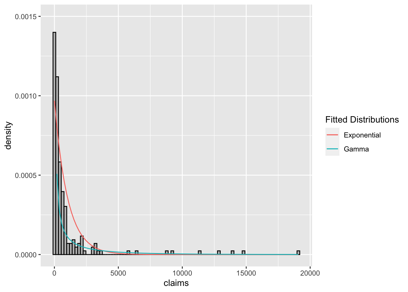
Figure 2.5: Histogram of claim sizes with fitted exponential and gamma distributions.
library(actuar)
# MME of mu and sigma for lognormal distribution

sigma_tilda <- sqrt(log(  var(dat$claims)/mean(dat$claims)^2 +1  ))  # gives \tilde\sigma
mu_tilda <- log(mean(dat$claims)) - sigma_tilda^2/2      # gives \tilde\mu

# MME of alpha and lambda for Pareto distribution
alpha_tilda <- 2*var(dat$claims)/mean(dat$claims)^2 * 1/(var(dat$claims)/mean(dat$claims)^2 - 1) #/tilde/alpha
lambda_tilda <- mean(dat$claims)*(alpha_tilda -1)


ggplot(dat) + geom_histogram(aes(x = claims, y = ..density..), bins = 90 , fill = "grey", color = "black") +
  stat_function(fun=dlnorm, geom ="line", args = list(meanlog = mu_tilda, sdlog = sigma_tilda), aes(colour = "Lognormal")) +
  stat_function(fun=dpareto, geom ="line", args = list(shape = alpha_tilda, scale = lambda_tilda), aes(colour = "Pareto")) +
  scale_color_discrete(name="Fitted Distributions")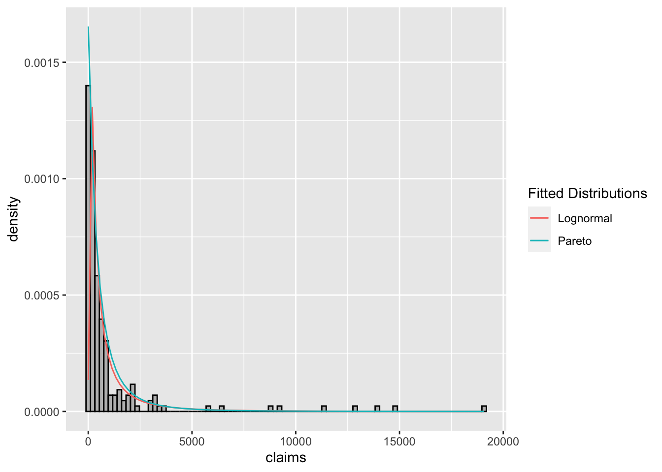
Figure 2.6: Histogram of claim sizes with fitted lognormal and pareto distributions.
Let us plot the histogram of claim sizes with fitted exponential and gamma distributions in this interaction area. Note that the data set is stored in the variable dat.
The following code can be used to obtain the expected number of claims for the fitted exponential distribution and perform goodness-of-fit test.