บทที่ 3 อนุพันธ์ (Derivatives)
3.1 อนุพันธ์ (Derivatives)
จากตัวอย่าง 2.1 ในบทที่ 2 และเนื้อหาในเรื่อง limits เราจะเห็นว่า ความชันของเส้นสัมผัสกราฟของฟังก์ชัน \(y=f\left( x\right)\) ณ จุด \(\left( x_{0},f\left( x_{0}\right) \right)\) บนกราฟ ก็คือ \(\underset{x\rightarrow x_{0}}{\lim}\frac{f\left( x\right) -f\left( x_{0}\right) }{x-x_{0}}\) นั่นเอง (ถ้า limit หาค่าได้)
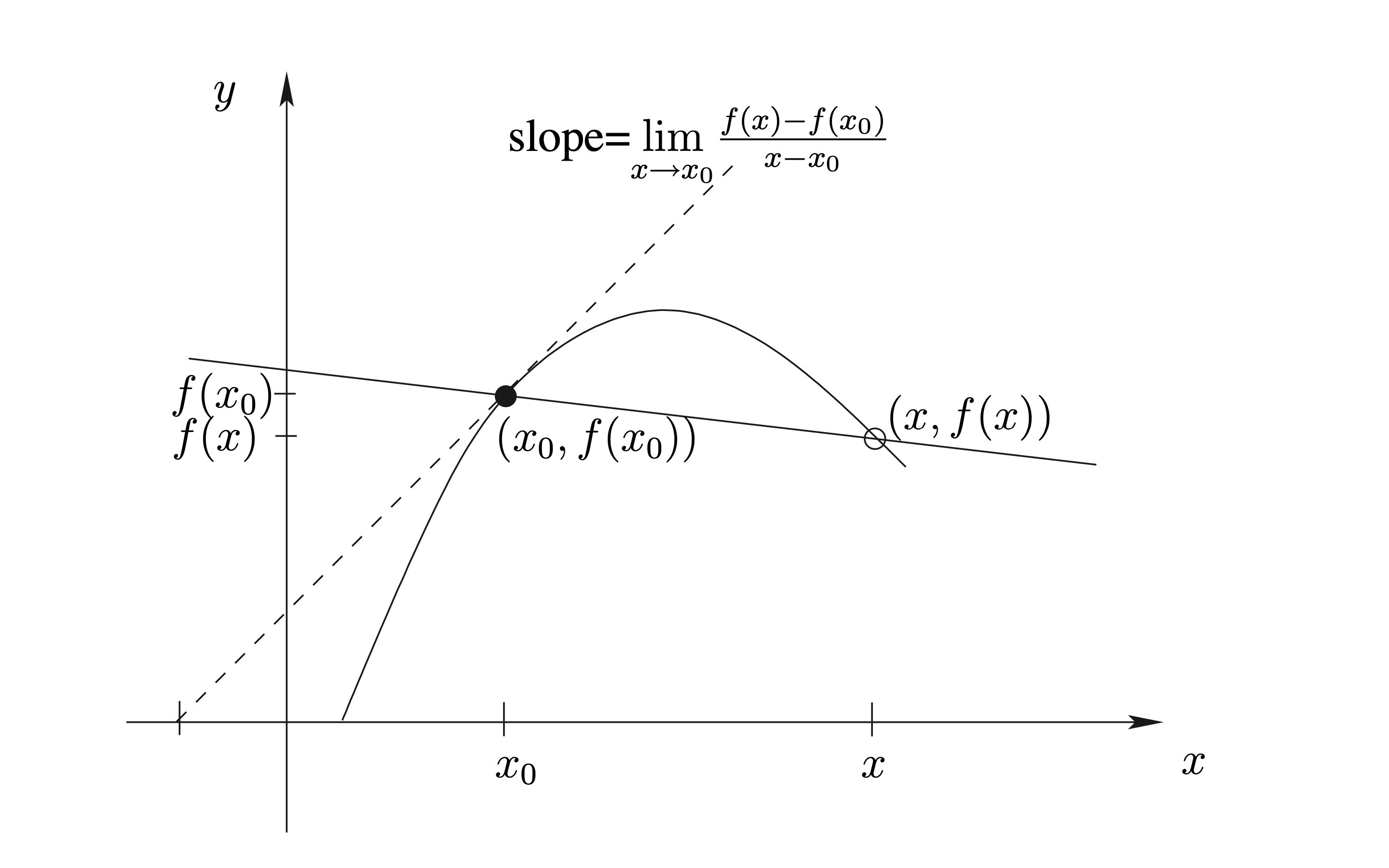
ปริมาณนี้มีความสำคัญ เพราะนำไปประยุกต์ใช้ได้มากมาย เราจึงกำหนดสัญลักษณ์และมีชื่อเรียกดังต่อไปนี้
นิยาม 3.1 ถ้า \(f : D_f \rightarrow \mathbb{R}\) โดยที่ \(D_f \subseteq \mathbb{R}\) และถ้า \(\underset{x \rightarrow x_0}{\lim} \frac{f(x)-f(x_0)}{x- x_0}\) หาค่าได้แล้ว เรียกค่าของ limit นี้ว่า “อนุพันธ์ (derivative) ของ \(f\) ที่ \(x_0\)” และแทนด้วยสัญลักษณ์ \(f'(x_0)\)
เนื่องจากแต่ละ function \(g\) และแต่ละ \(x_0\) จะมี \(\underset{x \rightarrow x_0}{\lim}g(x)\) ได้ค่าเดียว ดังนั้น \(f'\) จึงเป็น function เรียกว่า “อนุพันธ์ (derivative)” ของ \(f\)
ในการเขียนนิยามของ \(f'(x)\) เพื่อใช้เป็นสูตรทั่วไปสำหรับ function \(f'\) เราเปลี่ยนตัวแปรเสียใหม่ ดังแสดงในรูป
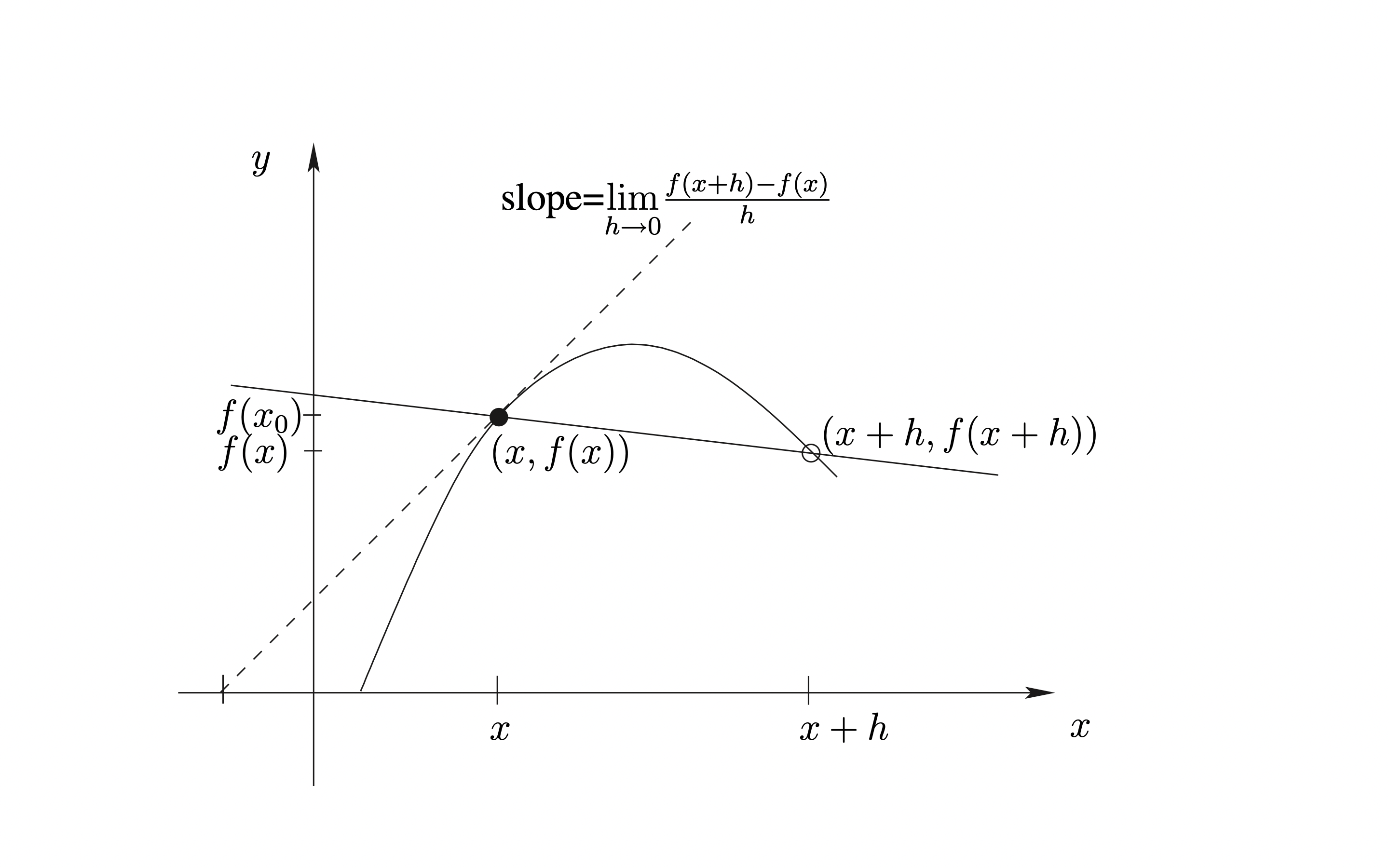
จะได้ว่า
ตัวอย่าง 3.1 จงหาสมการของเส้นสัมผัสกราฟ \(y = -x^2 + 6x -2\) ณ จุด \(P_0(2,6)\)
วิธีทำ ให้ \(f(x) = -x^2 + 6x -2\) จะได้ค่าความชันของเส้นสัมผัส ณ จุด \((x,f(x))\) คือ \(f'(x)\) ซึ่งเท่ากับ \[\begin{equation} \begin{aligned} \underset{h \rightarrow 0}{\lim}\frac{f(x+h) - f(x)}{h} &= \underset{h \rightarrow 0}{\lim}\frac{\left[-(x+h)^2 + 6(x+h)-2 \right]- \left[ -x^2 + 6x -2 \right] }{h} \\ &=\underset{h \rightarrow 0}{\lim}\frac{-2xh-h^2+6h}{h} \\ &=\underset{h \rightarrow 0}{\lim}(-2x-h+6) \leftarrow \boxed{\mbox{ อย่าเขียน $\underset{h \rightarrow 0}{\lim}-2x-h+6$}}\\ &=-2x+6 \end{aligned} \end{equation}\] ดังนั้น ความชันของเส้นสัมผัส ณ จุด \((2,6)\) คือ \(f'(2) = -2 \cdot 2 + 6 =2\) เส้นสัมผัสจึงมีสมการเป็น \(y - 6 = 2(x-2)\)
อัตราส่วน \(\displaystyle\frac{f(x+h) - f(x)}{h}\) คือ อัตราส่วนของค่า function
ที่เปลี่ยนไป (จาก \(f(x_0)\) กลายเป็น \(f(x)\)) ต่อค่าตัวแปรต้นที่เปลี่ยนไป (จาก \(x_0\)
กลายเป็น \(x\)) เรียกคำนี้ว่า “อัตราการเปลี่ยนแปลงเฉลี่ย (average rate of change)
ของ \(f(x)\) เทียบกับ \(x\)” คำว่าเฉลี่ยน แสดงถึงการคิดการเปลี่ยนแปลงบน ‘ช่วง’
แต่
\(\displaystyle\underset{x \rightarrow x_0}{\lim}\frac{f(x) - f(x_0)}{x-x_0}\)
เป็นการหา “แนวโน้ม” ของอัตราการเปลี่ยนแปลงเฉลี่ย เมื่อ \(x\) กับ \(x_0\) อยู่ใกล้กันมากๆ
จนแทบจะเป็นจุดเดียวกัน เราจึงเรียกค่านี้ว่า “อัตราการเปลี่ยนแปลงขณะหนึ่ง (instantaneous
rate of change) ของ \(f(x)\) เทียบกับ \(x\)”
สัญลักษณ์อื่นๆ สำหรับ derivatives ได้แก่
ถ้า \(f'(x_0)\) หาค่าได้ เรากล่าวว่า function \(f\) “หาอนุพันธ์ได้ (differentiable) ที่ \(x_0\)” ถ้า \(f'(x_0)\) หาค่าได้สำหรับทุกๆ \(x\) ในเซต \(S\) เรากล่าวว่า function \(f\) “หาอนุพันธ์บน \(S\) (differentiable on \(S\))” ถ้า \(f'(x_0)\) หาค่าได้สำหรับทุกๆ จำนวนจริง \(x\) เรากล่าวว่า function \(f\) “หาอนุพันธ์ได้ (differentiable)”
3.2 การคำนวณหาอนุพันธ์
ตัวอย่าง 3.2 จงหา derivative ต่อไปนี้
\(f'(x)\) เมื่อ \(f(x) = x^2\)
\(f'(2)\) เมื่อ \(f(x) = \sqrt{x}\)
\(\frac{ds(t)}{dt}|_{t=t_0}\) เมื่อ \(s(t) = \frac{1}{t}\)
วิธีทำ ใช้นิยามข้างต้นหา derivative ได้ดังนี้
เมื่อ \(f(x) = x^2\) จะได้ \[\begin{equation} \begin{aligned} f'(x) &= \underset{h \rightarrow 0}{\lim}\frac{f(x+h) - f(x)}{h} \\ &= \underset{h \rightarrow 0}{\lim}\frac{(x+h)^2-x^2}{h} \\ &= \underset{h \rightarrow 0}{\lim}\frac{(x^2+2xh+h^2)-x^2}{h} \\ &= \underset{h \rightarrow 0}{\lim}\frac{2xh+h^2}{h} \\ &= \underset{h \rightarrow 0}{\lim}2x + h \\ &= 2x \end{aligned} \end{equation}\]
เมื่อ \(f(x) = \sqrt{x}\) จะได้ \[\begin{equation} \begin{aligned} f'(2) &= \underset{h \rightarrow 0}{\lim}\frac{f(2+h) - f(2)}{h} \\ &= \underset{h \rightarrow 0}{\lim}\frac{\sqrt{2+h} - \sqrt{2}}{h} \\ &= \underset{h \rightarrow 0}{\lim}\frac{(\sqrt{2+h} - \sqrt{2}) \cdot (\sqrt{2+h} + \sqrt{2})}{h \cdot (\sqrt{2+h} + \sqrt{2})} \\ &= \underset{h \rightarrow 0}{\lim}\frac{(2+h)-2}{h\cdot (\sqrt{2+h} + \sqrt{2})} \\ &= \underset{h \rightarrow 0}{\lim}\frac{1}{(\sqrt{2+h} + \sqrt{2})} \\ &= \frac{1}{2\sqrt{2}} \end{aligned} \end{equation}\]
เมื่อ \(s(x) = \frac{1}{t}\) จะได้ \[\begin{equation} \begin{aligned} s'(t)|_{t=t_0} &= \underset{h \rightarrow 0}{\lim}\frac{s(t_0+h) - s(t_0)}{h} \\ &= \underset{h \rightarrow 0}{\lim}\frac{\frac{1}{t_0+h}-\frac{1}{t_0}}{h} \\ &= \underset{h \rightarrow 0}{\lim}\frac{t_0-(t_0+h)}{t_0(t_0+h)h} \\ &= \underset{h \rightarrow 0}{\lim}\frac{-h}{t_0(t_0+h)h} \\ &= \underset{h \rightarrow 0}{\lim}\frac{-1}{t_0(t_0+h)} \\ &= \frac{-1}{t_0^2} \end{aligned} \end{equation}\]
ตัวอย่าง 3.3 จงหาเซต \(S\) ที่ใหญ่ที่สุดที่ทำให้ function \(f(x) = \sqrt{x}\) หาอนุพันธ์ได้บน \(S\)
วิธีทำ พิจารณาจำนวนจริง \(x\) ที่ทำให้ \(f'(x)\) หาค่าได้ เนื่องจาก \[f'(x) = \frac{1}{2\sqrt{x}} \text{ ถ้า } x>0\] ในกรณีที่ \(x \le 0\) จะได้ว่า \(f(x)\) ไม่นิยาม จึงหาอนุพันธ์ที่ \(x\) ไม่ได้ และในกรณีที่ \(x=0\) จะได้ว่า \[\begin{equation} \begin{aligned} \underset{h \rightarrow 0}{\lim}\frac{1}{\sqrt{x+h}+\sqrt{x}} &=\underset{h \rightarrow 0}{\lim}\frac{1}{\sqrt{0+h}+\sqrt{0}} \\ &=\underset{h \rightarrow 0}{\lim}\frac{1}{\sqrt{h}} \end{aligned} \end{equation}\] ซึ่งหาค่าไม่ได้ ดังนั้นจึงได้ว่า เซตที่ใหญ่ที่สุดที่ทำให้ function \(f(x) = \sqrt{x}\) หาอนุพันธ์ได้บน \(S\) คือ ช่วงเปิด \((0,\infty)\)
3.3 สูตรสำหรับหาอนุพันธ์
ทฤษฎี 3.1 ถ้า \(c\) เป็นจำนวนจริง (real number) และ \(n\) เป็นจำนวนจริงใดๆ แล้ว function \(f(x) = c\) เป็น function ที่ differentiable และ function \(g(x) = x^n\) เป็น function ที่ differentiable บนช่วงเปิดในโดเมนของมัน และ
\(\frac{dc}{dx} = 0\)
\(\frac{dx^n}{dx} = n x^{n-1}\)
ทฤษฎี 3.2 ถ้า \(f\) และ \(g\) เป็น function ซึ่ง differentiable ที่ \(x_0\) และ \(c\) เป็นค่าคงที่จริง แล้ว
\((f+g)'(x_0) = f'(x_0) + g'(x_0)\)
\((cf)'(x_0) = cf'(x_0)\)
\((f-g)'(x_0) = f'(x_0) - g'(x_0)\)
\((f \cdot g)'(x_0) = f'(x_0) \cdot g(x_0) + f(x_0)\cdot g'(x_0)\)
\((\frac{f}{g})'(x_0) = \frac{f'(x_0) \cdot g(x_0) - f(x_0)\cdot g'(x_0)}{(g(x_0))^2}\)
ตัวอย่าง 3.4 จงหา derivative ของแต่ละ function ต่อไปนี้ เทียบกับตัวแปรต้นของมัน
\(f(x) = 5x^4\)
\(f(x) = 6x^{11} + 9\)
\(s(t) = 3t^8 - 2t^5 + 6t + 1\)
\(g(x) = \left( x^2 - 1 + \frac{1}{2x} \right) \left(2x - 1 + \frac{1}{x^2} \right)\)
\(h(x) = \frac{x^2 -1}{x^4 + 1}\)
วิธีทำ ใช้สูตรในทฤษฎีบทข้างต้นหา derivative ได้ดังนี้
\[\begin{equation} \begin{aligned} f(x) &= 5x^4 \\ f'(x) &= \frac{d}{dx}(5 \cdot x^4) \\ &= 5 \frac{d}{dx}( x^4) = 5 \cdot 4x^3 = 20x^3 \end{aligned} \end{equation}\]
\[\begin{equation} \begin{aligned} f(x) &= 6x^{11} + 9 \\ f'(x) &= \frac{d}{dx}(6x^{11} + 9) \\ &= 5 \frac{d}{dx}(6x^{11}) + \frac{d}{dx}9\\ &= 66x^{10} \end{aligned} \end{equation}\]
\[\begin{equation} \begin{aligned} s(t) &= 3t^8 - 2t^5 + 6t + 1 \\ s'(t) &= \frac{d}{dt}(3t^8 - 2t^5 + 6t + 1) \\ &= 24t^7 - 10t^4 + 6 \end{aligned} \end{equation}\]
\[\begin{equation} \begin{aligned} g(x) &= \left( x^2 - 1 + \frac{1}{2x} \right) \left(2x - 1 + \frac{1}{x^2} \right) \\ g'(x) &= \frac{d}{dx}\left( x^2 - 1 + \frac{1}{2x} \right)\left(2x - 1 + \frac{1}{x^2} \right) + \left( x^2 - 1 + \frac{1}{2x} \right) \frac{d}{dx} \left(2x - 1 + \frac{1}{x^2} \right)\\ &= \left(2x - \frac{1}{2}x^{-1} \right)\left(2x - 1 + \frac{1}{x^2} \right) + \left( x^2 - 1 + \frac{1}{2x} \right) \left(2x -2x^{-3} \right) \end{aligned} \end{equation}\]
\[\begin{equation} \begin{aligned} h(x) &= \frac{x^2 -1}{x^4 + 1} \\ h'(x) &= \frac{(x^4 + 1) \frac{d}{dx}(x^2 -1) - (x^2 -1)\frac{d}{dx}(x^4 + 1) }{(x^4 + 1)^2}\\ &= \frac{(x^4 + 1) (2x) - (x^2 -1)(4x^3) }{(x^4 + 1)^2} \end{aligned} \end{equation}\]
ตัวอย่าง 3.5 จงหา \(f'(0)\) เมื่อ \(f(x) = (x^6 - x^5-x^4-x^3)(x^5-x^4-x^3-x^2)\)
วิธีทำ จาก \(f(x) = (x^6 - x^5-x^4-x^3)(x^5-x^4-x^3-x^2)\) จะได้ \[f'(x) = (x^6 - x^5-x^4-x^3)(5x^4-4x^3-3x^2-2x) + (x^5-x^4-x^3-x^2)(6x^5 - 5x^4-4x^3-3x^2)\] ดังนั้น \(f'(0) = 0\)
3.4 อนุพันธ์อันดับสูง (High Order Derivatives)
ถ้า \(f\) เป็น function ที่หา derivative ได้ และ \(f'\) ก็เป็น function ที่หา derivative ได้อีก เราเรียก \((f')'\) ว่า “อนุพันธ์อันดับสอง (second derivative) ของ \(f\)” เขียนแทนด้วย \(f''\) ในทำนองเดียวกัน เราจะมี “อนุพันธ์อันดับสาม (third derivative) ของ \(f\)” เขียนแทนด้วย \(f'''\) ฯลฯ สำหรับอนุพันธ์อันดับ \(n\) (\(n\)th derivative) ของ \(f\) โดยที่ \(n \ge 4\) เราเขียนแทนด้วย \(f^{(n)}\) นอกจากนี้เราใช้สัญลักษณ์ \(\frac{d^nf(x)}{dx}\) แทน \(n\)th derivative ของ \(f\) และ \(\frac{d^nf(x)}{dx}|_{x=x_0}\) แทน \(n\)th derivative ของ \(f\) ที่ \(x_0\) (ซึ่งคือ \(f^{(n)}(x_0)\) นั่นเอง)
ถ้าให้ \(y= f(x)\) เราสามารถใช้สัญลักษณ์ \(y', y'', y''', y^{(4)}, \ldots, y^{(n)}\) หรือ \(\frac{dy}{dx}, \frac{d^2y}{dx^2}, \frac{d^3y}{dx^3}, \frac{d^4y}{dx^4}, \ldots, \frac{d^ny}{dx^n}\) แทนอนุพันธ์อันดับที่ \(1,2,3,4,\ldots,n\) ตามลำดับ และแทนค่าอนุพันธ์ที่ \(x_0\) ด้วย \(\frac{d^ny}{dx^n}|_{x=x_0}\)
ด้วยหลักการเดียวกัน “อนุพันธ์อันดับหนึ่ง (first derivative) ของ \(f\)” ก็คือ อนุพันธ์ของ \(f\) นั่นเอง
ตัวอย่าง 3.6 จงหาอนุพันธ์ทั้งหมดของ \(f(x) = x^n\) เมื่อ \(n > 1\)
วิธีทำ จาก \(f(x) = x^n\) จะได้ \[\begin{equation} \begin{aligned} f'(x) &= n x^{n-1} \\ f''(x) &= n(n-1) x^{n-2} \\ f'''(x) &= n(n-1)(n-2) x^{n-3} \\ f^{(4)}(x) &= n(n-1)(n-2)(n-3) x^{n-4} \\ &\vdots \\ f^{(n)}(x) &= n! \\ f^{(k)}(x) &= 0 \text{ เมื่อ } k \ge n \end{aligned} \end{equation}\]
3.5 การตีความอนุพันธ์ (Interpretation of Derivatives)
3.5.1 อนุพันธ์ในเชิงความชัน (Derivatives as Slopes)
ในกรณีที่เราลงจุดกราฟ (plot graph) ของฟังก์ชัน เราได้ทราบมาแล้วว่า อนุพันธ์ของฟังก์ชัน \(f\) ที่จุด \(x\) ใดๆ ก็คือความชันของเส้นสัมผัสกราฟ (เรียกว่าความชันของกราฟ) ของฟังก์ชัน \(f\) ที่จุด \((x,f(x))\) นั่นเอง ความจริงข้อนี้สามารถนำไปใช้แก้ปัญหาเกี่ยวกับกราฟของฟังก์ชันได้
ตัวอย่าง 3.7 จงพิจารณาว่ามีเส้นสัมผัสกราฟของฟังก์ชัน \(\displaystyle f(x)=\frac{x}{x+1}\) ที่ตั้งฉากกันหรือไม่
วิธีทำ เราทราบว่าเส้นตรงสองเส้นตั้งฉากกันก็ต่อเมื่อ ผลคูณของความชันของเส้นตรงทั้งสองเท่ากับ \(-1\) พิจารณาความชันของเส้นสัมผัสกราฟของฟังก์ชัน \(\displaystyle f(x)=\frac{x}{x+1}\) ที่จุด \((x,f(x))\) ใดๆ จะได้ว่า ความชันดังกล่าวมีค่าเท่ากับ \(\displaystyle f'(x)=\frac{d}{dx}\left(\frac{x}{x+1}\right)=\frac{1}{(x+1)^2}\) ฉะนั้น ความชันของเส้นสัมผัสกราฟนี้ที่จุดใดๆ จึงมีค่าเป็นบวกเสมอ จึงสรุปได้ว่า กราฟของฟังก์ชันนี้ไม่มีเส้นสัมผัสคู่ใดตั้งฉากกัน เพราะผลคูณของความชันของเส้นสัมผัสเป็นจำนวนจริงบวกเสมอ ไม่สามารถเป็น \(-1\) ได้
ตัวอย่าง 3.8 ภูเขาจำลองในพิพิธภัณฑ์วิทยาศาสตร์แห่งหนึ่ง เกิดจากการหมุนของพาราโบลาคว่ำรอบแกนสมมาตรของมัน โดยที่ฐานของภูเขาจำลองเป็นรูปวงกลมรัศมี 5 เมตร และยอดเขาอยู่สูงจากฐานเป็นระยะทาง 8 เมตร บนยอดเขาติดตั้งโคมไฟ ณ ตำแหน่งสูงจากยอดเขาขึ้นไปอีก 0.5 เมตร เมื่อเปิดโคมไฟ แสงไฟจากโคมจะทำให้พื้นบริเวณรอบๆ ภูเขาจำลองที่ไม่ถูกภูเขาจำลองบัง สว่างขึ้น จงหาว่าบริเวณที่สว่างดังกล่าว เป็นบริเวณบนพื้นภายนอกวงกลมรัศมีเท่าใด
จากโจทย์จำลองรูปได้ดังภาพ 1.3 ในที่นี้สมมุติว่าแหล่งกำเนิดแสงเป็นจุด จะเห็นว่า แนวแบ่งส่วนมืดและส่วนสว่างจะผ่านจุดกำเนิดแสง และอยู่ในแนวเส้นสัมผัสผิวของพาราโบลาด้วย ให้จุดกึ่งกลางฐานของภูเขาจำลองเป็นจุดกำเนิด และสมมุติให้ \(f(x)=a-kx^2\) เป็นสมการของรูปพาราโบลา จากเงื่อนไขความกว้างและความสูงของภูเขาจำลอง จะได้ว่า \(f(0)=8\) และ \(f(5)=0\) ซึ่งทำให้ \(a=8\) และ \(k=8/25\) ดังนั้น \(f(x)=8-8x^2/25\) ให้ \((x,f(x))\) เป็นจุดที่แนวแบ่งส่วนมืดและส่วนสว่างสัมผัสกับพาราโบลา จะได้ว่า ความชันของเส้นสัมผัสกราฟที่จุดดังกล่าวเท่ากับ \(f'(x)=-16x/25\) แต่เส้นสัมผัสนี้ผ่านจุดกำเนิดแสง \((0,8.5)\) และจุด \((x,f(x))=(x,8-8x^2/25)\) จึงได้ว่า มีความชันเป็น \(\displaystyle\frac{8-8x^2/25-8.5}{x-0}\) นั่นคือ \(\displaystyle\frac{8-8x^2/25-8.5}{x-0}=-16x/25\) หรือ \(x=5/4\) ดังนั้นความชันของเส้นสัมผัสเท่ากับ \(-16\times(5/4)/25=-4/5\) ถ้าบริเวณบนพื้นที่สว่าง เป็นบริเวณภายนอกวงกลมรัศมี \(r\) จะได้ว่า เส้นสัมผัสข้างต้น ต้องผ่านจุด \((r,0)\) ด้วย นั่นคือความชันจะเท่ากับ \(\displaystyle\frac{0-8.5}{r-0}\) ซึ่งทำให้ \(\displaystyle\frac{0-8.5}{r-0}=-4/5\) หรือ \(r=10.625\) นั่นคือ บริเวณที่สว่าง เป็นบริเวณบนพื้นภายนอกวงกลมรัศมี 10.625 เมตร
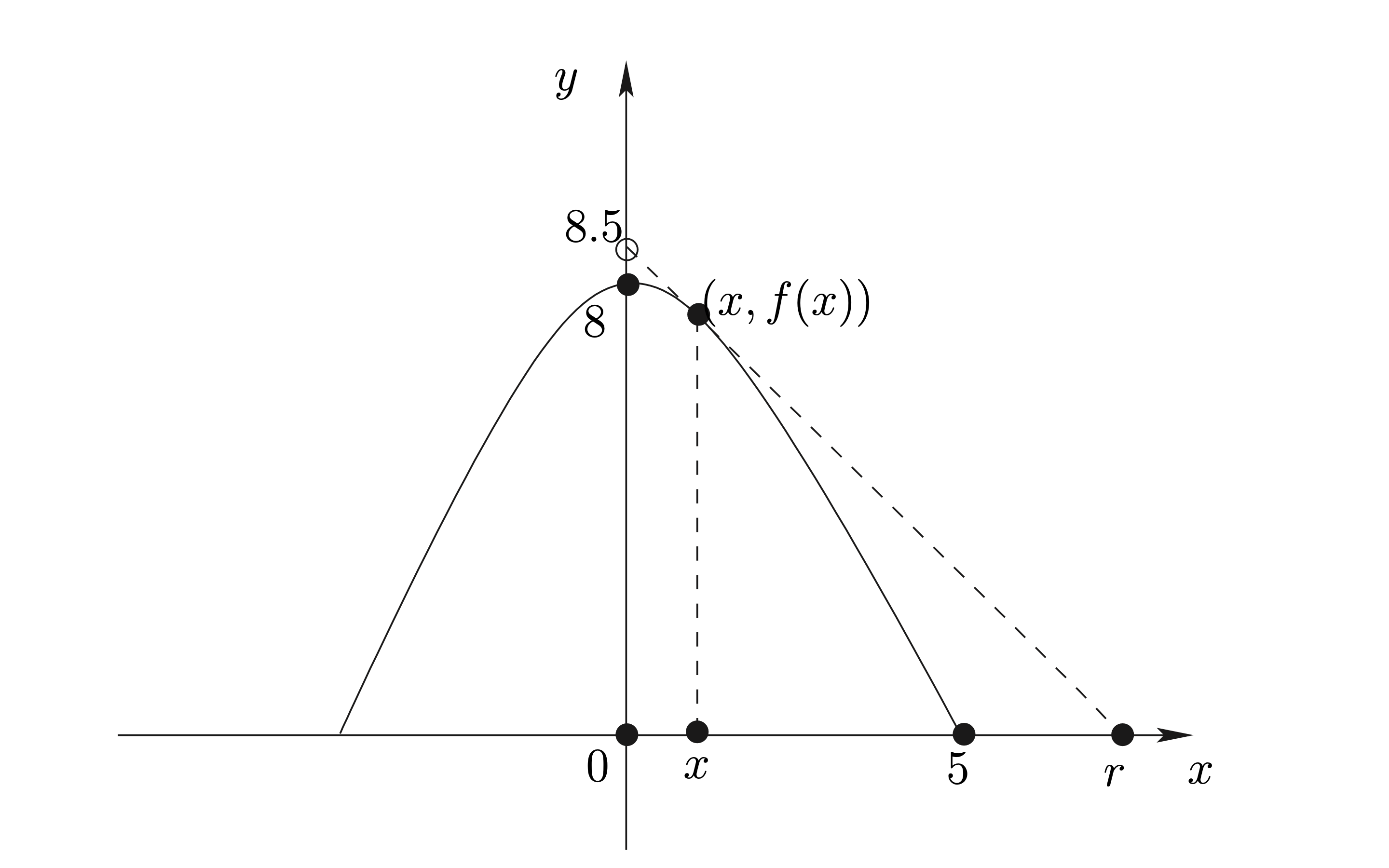
Figure 3.1: รูปภาพสำหรับตัวอย่างข้างต้น
3.5.2 อนุพันธ์ในเชิงอัตราเร็ว (Derivatives as Speeds)
ถ้าพิจารณาการเคลื่อนที่ของวัตถุ โดยให้ \(f(t)\) เป็นระยะทางที่วัตถุเคลื่อนที่ได้ ณ เวลา \(t\) เราจะได้ว่า \(f'(t)\) ก็คืออัตราเร็ว ณ เวลา \(t\) ซึ่งเรียกว่า อัตราเร็วชั่วขณะ (instantaneous speed) ในขณะที่ปริมาณ \(\displaystyle \frac{f(s)-f(t)}{s-t}\) เรียกว่า อัตราเร็วเฉลี่ยของวัตถุ ในช่วงเวลา ตั้งแต่ \(s\) ถึง \(t\)
ตัวอย่าง 3.9 วัตถุเคลื่อนที่เป็นเวลานาน 1 นาที ตามสมการ \(s=0.5t+0.1t^2\) เมื่อ \(t\) คือเวลาเป็นวินาที และ \(s\) คือระยะทางที่เคลื่อนที่ได้เป็นเมตร จงหา
อัตราเร็วเฉลี่ยของวัตถุในช่วง 10 วินาทีแรก และในช่วง 10 วินาทีถัดไป
อัตราเร็วของวัตถุ ณ วินาทีที่ 10 และ ณ วินาทีที่ 20
วิธีทำ
(1) อัตราเร็วเฉลี่ยของวัตถุในช่วง 10 วินาทีแรก เท่ากับ
\(\displaystyle\frac{s(10)-s(0)}{10-0}
=\frac{(0.5\times10+0.1\times10^2)-(0.5\times0+0.1\times0^2)}{10-0}=1.5\)
เมตรต่อวินาที
อัตราเร็วเฉลี่ยของวัตถุในช่วง 10 วินาทีถัดไป เท่ากับ
\(\displaystyle\frac{s(20)-s(10)}{20-10}
=\frac{(0.5\times20+0.1\times20^2)-(0.5\times10+0.1\times10^2)}{20-10}=3.5\)
เมตรต่อวินาที
(2) เนื่องจาก
\(\displaystyle\frac{d}{dt}\left(0.5t+0.1t^2\right)=0.5+0.2t\)
ดังนั้น อัตราเร็วของวัตถุ ณ วินาทีที่ 10 เท่ากับ
\(\displaystyle\left.\frac{ds}{dt}\right|_{t=10}
=\left.\frac{d}{dt}\left(0.5t+0.1t^2\right)\right|_{t=10}=0.5+0.2\times10=2.5\)
เมตรต่อวินาที
และ อัตราเร็วของวัตถุ ณ วินาทีที่ 20 เท่ากับ
\(\displaystyle\left.\frac{ds}{dt}\right|_{t=20}
=\left.\frac{d}{dt}\left(0.5t+0.1t^2\right)\right|_{t=20}=0.5+0.2\times20=4.5\)
เมตรต่อวินาที
3.5.3 อนุพันธ์ในเชิงอัตราการเปลี่ยนแปลง (Derivatives as Rates of Change)
เราจะเห็นได้ชัดจากนิยามของอนุพันธ์ว่า ในกรณีของฟังก์ชันทั่วๆ ไป อนุพันธ์ของฟังก์ชัน ก็คืออัตราการเปลี่ยนแปลงของค่าฟังก์ชัน เทียบกับตัวแปรต้นของมันนั่นเอง
ตัวอย่าง 3.10 เมื่อใช้เครื่องสูบลม สูบลมเข้าไปในลูกโป่ง เราอาจประมาณได้ว่า ณ ขณะเวลาใดๆ ลูกโป่งมีรูปร่างเป็นรูปทรงกลม จงหาอัตราการเพิ่มขึ้นของปริมาตรของลูกโป่ง ต่อหนึ่งหน่วยรัศมีที่เพิ่มขึ้นของลูกโป่ง ขณะที่ลูกโป่งมีรัศมี 10 เซนติเมตร
วิธีทำ ให้ \(r\) เป็นรัศมีของลูกโป่ง และ \(V\) เป็นปริมาตรของลูกโป่ง จากข้อสมมุติว่าลูกโป่งเป็นทรงกลม จะได้ว่า \(V=4\pi r^3/3\) ดังนั้น อัตราการเปลี่ยนแปลงของปริมาตรของลูกโป่งเทียบกับรัศมีเท่ากับ \(\displaystyle\frac{dV}{dr}=12\pi r^2/3=4\pi r^2\) ลูกบาศก์หน่วยต่อหน่วย นั่นคือ ขณะที่ลูกโป่งมีรัศมี 10 เซนติเมตร มันจะมีปริมาตรเพิ่มขึ้นในอัตรา \(4\times\pi\times10^2\approx1256\) ลูกบาศก์เซนติเมตรต่อเซนติเมตร หรือประมาณ \(1.256\) ลิตรต่อรัศมีที่เพิ่มขึ้น 1 เซนติเมตร
3.5.4 แบบฝึกหัด (Exercises)
จงหาอนุพันธ์ต่อไปนี้ ถ้าอนุพันธ์ดังกล่าวหาค่าได้ ในกรณีที่หาค่าไม่ได้ ให้ระบุว่าหาค่าไม่ได้
\(\displaystyle f'(x)\) เมื่อ \(f(x)=g(x)h(x)k(x)\)
\(\displaystyle f^{(n)}(0)\) เมื่อ \(\displaystyle f(x)=\sum_{i=1}^k x^i\) โดยที่ \(k\) และ \(n\) เป็นจำนวนนับ
\(\displaystyle\frac{d}{dt}\frac1{1-t}\) และ \(\displaystyle\frac{d^2}{dt^2}\frac1{1-t}\)
\(\displaystyle\frac{d}{dt}\frac{f(t)}t\) เมื่อ \(f\) เป็นฟังก์ชันซึ่ง \(\displaystyle\frac{d}{dt}f(t)=\frac{f(t)}t\) สำหรับทุกๆ \(t\neq0\)
\(f'(-1)\), \(f'(-\frac23)\), \(f'(0)\), \(f'(1)\) เมื่อ \(f(x)=x\sqrt{1+x}\)
\(\displaystyle\left.\frac d{dx}\,\frac x{\sqrt{1+x}-\sqrt{1-x}}\right|_{x=0}\)
\(\displaystyle\frac {dy}{dx}\;\), \(\displaystyle\left.\frac {dy}{dx}\,\right|_{x=0}\), \(\displaystyle\left.\frac {dy}{dx}\,\right|_{x=0.25}\), \(\displaystyle\left.\frac {dy}{dx}\,\right|_{x=1}\) เมื่อ \(\displaystyle y=\frac{1-\sqrt x}{\sqrt{1-x}}\)
\(\displaystyle\frac d{dx}\,\left(x^2\sqrt{1+x}\right)\)
\(\displaystyle\frac {d^2y}{dx^2}\) เมื่อ \(y=(1+x^2)\sqrt{1-2x}\) ( หาอนุพันธ์ของ \(\sqrt{1-2x}\) และ \(1/\sqrt{1-2x}\) ก่อน)
\(\displaystyle\frac {d^{10}y}{dx^{10}}\) เมื่อ \(y=\left(x^5-x^4-x^3-x^2-x-1\right)\left(x^5+2x^4+2x^3+2x^2+2x+2\right)\)
จงตอบคำถามต่อไปนี้
จงหาความชันของกราฟของสมการ \(y=x^3-3x\) ณ ตำแหน่งซึ่ง \(x=2\)
จงหาจุดบนกราฟ \(y=x^3-3x\) ซึ่งมีเส้นสัมผัสกราฟที่ขนานกับเส้นสัมผัส ณ จุดซึ่ง \(x=a\) เมื่อ \(a\) เป็นจำนวนจริงใดๆ
จงหาจุดบนกราฟ \(y=x^3-3x\) ซึ่งมีเส้นสัมผัสกราฟที่ตั้งฉากกับเส้นสัมผัส ณ จุดซึ่ง \(x=a\) เมื่อ \(a\) เป็นจำนวนจริงใดๆ
3.6 กฎลูกโซ่ (The Chain Rule)
การทราบข้อมูลของ derivative ของฟังก์ชัน \(f\) และฟังก์ชัน \(g\) ทำให้เราสามารถหา derivative ของผลบวก \(f+g\) ผลคูณ \(fg\) และผลหาร \(f/g\) ของฟังก์ชัน ทั้งสองได้ ข้อมูลนี้ยังใช้หา derivative ของฟังก์ชันประกอบ \(f\circ g\) ภายใต้เงื่อนไขที่เหมาะสมได้ เราเรียกวิธีการหา derivative ของฟังก์ชัน ประกอบว่า chain rule โดยมีแนวคิดสำคัญคือ การสร้างตัวแปรใหม่ขึ้นมาช่วย ในการคำนวณ ดังรายละเอียดในทฤษฏีบทต่อไปนี้
ทฤษฎี 3.3 ถ้าฟังก์ชัน \(g\) หา derivative ได้ที่จุด \(x\) และฟังก์ชัน \(f\) หา derivative ได้ที่จุด \(g(x)\) แล้ว ฟังก์ชันประกอบ \(f \circ g\) หา derivative ได้ที่จุด \(x\) ยิ่งกว่านั้น ถ้า \[y = f(g(x)) \quad \text{และ} \quad u = g(x)\] แล้ว \(y=f(u)\) และ \[\label{E:chain1} \boxed{ \frac{dy}{dx} = \frac{dy}{du} \cdot \frac{du}{dx} }\]
ตัวอย่างต่อไปนี้แสดงให้เห็นถึงการใช้ chain rule หา derivative ของฟังก์ชัน
ตัวอย่าง 3.11 พิจารณาฟังก์ชัน \(y = \frac{1}{x^2+1}\) กำหนดให้ \(u = x^2+1\) จงหา \(\frac{dy}{dx}\)
วิธีทำ ในที่นี้ \(y = \frac{1}{u}\) เราใช้ chain rule ได้ว่า \[\begin{equation} \begin{aligned} \frac{dy}{dx} &= \frac{dy}{du} \cdot \frac{du}{dx} \\ &= \frac{d}{du}\left[\frac{1}{u}\right] \cdot \frac{d}{dx}[x^2+1] \\ &= \left(-\frac{1}{u^2}\right) \cdot (2x) \\ &= -\frac{1}{(x^2+1)^2} \cdot (2x) \\ &= -\frac{2x}{(x^2+1)^2} \end{aligned} \end{equation}\] นั่นคือ \(\displaystyle \frac{dy}{dx} = -\frac{2x}{(x^2+1)^2}\)
ตัวอย่าง 3.12 กำหนดให้ \(y = u^{100}\) และ \(u = x^3 + x^2 + x + 1\) จงหา \(\frac{dy}{dx}\)
วิธีทำ ใช้ chain rule ได้ว่า \[\begin{equation} \begin{aligned} \frac{dy}{dx} &= \frac{dy}{du} \cdot \frac{du}{dx} \\ &= \frac{d}{du}[u^{100}] \cdot \frac{d}{dx}[x^3+x^2+x+1] \\ &= (100u^{99}) \cdot (3x^2+2x+1) \\ &= 100(x^3+x^2+x+1)^{99}(3x^2+2x+1) \end{aligned} \end{equation}\] นั่นคือ \(\displaystyle \frac{dy}{dx} = 100(x^3+x^2+x+1)^{99}(3x^2+2x+1)\)
ข้อสังเกต สูตรของกฎลูกโซ่สามารถเขียนได้ในอีกรูป ซึ่งสะดวกในการนำไปใช้ สังเกตว่า \(y = f(u)\) ดังนั้น \[\frac{dy}{dx} = \frac{d}{dx}[f(u)] \quad \text{และ} \quad \frac{dy}{du} = f'(u)\] สูตรของ chain rule จึงเขียนได้ว่า \[\label{E:chain2} \boxed{ \frac{d}{dx}[f(u)] = f'(u)\frac{du}{dx} }\] ซึ่งเขียนได้อีกรูปคือ \[\frac{d}{dx} f(g(x)) = f'(g(x))\cdot g'(x)\]
ตัวอย่าง 3.13 จงหา derivative ของฟังก์ชัน \(y = \sqrt{\frac{1}{2}x^2+x+1}\)
วิธีทำ เราแนะนำตัวแปร \(u = \frac{1}{2}x^2+x+1\) และใช้สูตร chain rule ได้ว่า \[\begin{equation} \begin{aligned} \frac{d}{dx} \left[\sqrt{\frac{1}{2}x^2+x+1} \right] &= \frac{d}{dx}[\sqrt{u}] \\ &= \frac{d}{du}\sqrt{u} \cdot \frac{du}{dx} \\ &= \frac{1}{2\sqrt{u}} \frac{du}{dx} \\ &= \frac{1}{2\sqrt{\frac{1}{2}x^2+x+1}} \frac{d}{dx} \left[\frac{1}{2}x^2+x+1\right] \\ &= \frac{1}{2\sqrt{\frac{1}{2}x^2+x+1}} \cdot (x+1) \\ &= \frac{x+1}{2\sqrt{\frac{1}{2}x^2+x+1}} \end{aligned} \end{equation}\] นั่นคือ \(\displaystyle \frac{dy}{dx} = \frac{x+1}{2\sqrt{\frac{1}{2}x^2+x+1}}\)
ตัวอย่าง 3.14 จงหาค่าของ \(f'(x^3+x)\) เมื่อกำหนดให้ \[\frac{d}{dx}[f(x^3+x)] = (3x^2+1)^2\]
วิธีทำ เราใช้ chain rule ได้ว่า \[\begin{equation} \begin{aligned} \frac{d}{dx}[f(x^3+x)] &= f'(x^3+x) \frac{d}{dx} [x^3+x] \\ &= f'(x^3+x) \cdot (3x^2+1) \end{aligned} \end{equation}\] ดังนั้น \[(3x^2+1)^2 = f'(x^3+x)\cdot(3x^2+1)\] หรือ \[f'(x^3+x) = 3x^2+1\] สังเกตความแตกต่างระหว่าง \(\displaystyle \frac{d}{dx} f(x^3+x)\) และ \(f'(x^3+x)\)
ตัวอย่าง 3.15 กำหนดให้ \(f(x) = |x|\) จงหา derivative ของฟังก์ชัน \(f\) ที่ \(x \ne 0\)
วิธีทำ ฟังก์ชัน \(f\) เขียนได้ว่า \[f(x) = |x| = \sqrt{x^2}\] ถ้า \(x\ne 0\) แล้ว \[\begin{equation} \begin{aligned} f'(x) &= \frac{d}{dx} \sqrt{x^2} \\ &= \frac{d}{du} [\sqrt{u}] \cdot \frac{d}{dx} [x^2] \\ &= \frac{1}{2\sqrt{u}} \cdot (2x) \\ &= \frac{1}{\sqrt{x^2}} \cdot x \\ &= \frac{x}{|x|} \end{aligned} \end{equation}\] นั่นคือ เมื่อ \(x\ne 0\) แล้ว \(\displaystyle f'(x) = \frac{x}{|x|}\)
3.6.1 แบบฝึกหัด
จงหา derivative ของฟังก์ชันต่อไปนี้
\(\displaystyle f(x) = \sqrt{1-x+x^2}\)
\(\displaystyle f(x) = \frac{1}{1+x+x^2}\)
\(\displaystyle f(x) = (2x+5)^3(3x-7)^5\)
\(\displaystyle f(x) = \frac{x^2+1}{x^3+x^2+1}\)
จงหา derivative ของฟังก์ชัน \[y = \sqrt{x + \sqrt[3]{3x + \sqrt[4]{4x}}}\]
กำหนดให้ \(f\) เป็นฟังก์ชันหา derivative ได้ และ \(g = f \circ f\) ถ้า \(f(1) = 1\), \(f(2) = 4\) และ \(f'(4) = 8\) จงหาค่าของ \(g'(1)\)
พิจารณาตารางค่าของฟังก์ชัน \(f, f'\), \(g, g'\) และ \(h, h'\) โดยที่ \(h=f\circ g\)
\(x\) \(f(x)\) \(g(x)\) \(h(x)\) \(f'(x)\) \(g'(x)\) \(h'(x)\) -1 0 1 2 2 0 2 0 3 -1 ? 1 1 ? 1 ? 0 0 ? ? 3 จงหาค่าของ \(h(0)\), \(f(1)\), \(h'(0)\), \(f'(1)\) และ \(g'(1)\)
จาก chain rule \[E:chain1\], \(\frac{dy}{dx} = \frac{dy}{du} \cdot \frac{du}{dx}\), จงหาสูตร ของ \(\displaystyle \frac{d^2y}{dx^2}\)
3.7 อนุพันธ์ของฟังก์ชันอินเวอร์ส (Derivatives of Inverse Functions)
นิยาม 3.2 ถ้าฟังก์ชัน \(f\) และ \(g\) สอดคล้องสมบัติ
\(g(f(x)) = x\) สำหรับ \(x\) ที่เป็นสมาชิกของโดเมนของ \(f\)
\(f(g(y)) = y\) สำหรับ \(y\) ที่เป็นสมาชิกของโดเมนของ \(g\)
เรากล่าวว่า \(f\) และ \(g\) เป็นฟังก์ชันอินเวอร์ส โดยที่ \(f\) เป็น ฟังก์ชันอินเวอร์สของ \(g\) และ \(g\) เป็นฟังก์ชันอินเวอร์ส ของ \(f\)
ถ้าเขียน \(f^{-1}\) แทน \(g\) และใช้สัญกรณ์ \(x\) แทนสมาชิกทั้งในโดเมนของ \(f\) และ \(f^{-1}\) สมมติว่าทั้งสองฟังก์ชันหา derivative ได้ ให้ \[y = f^{-1}(x)\] เราสามารถเขียนใหม่ได้ว่า \[x = f(y)\] หา derivative เทียบกับ \(x\) \[\begin{equation} \begin{aligned} \frac{d}{dx}[x] &= \frac{d}{dx}[f(y)] \\ &= f'(y) \cdot \frac{dy}{dx} \end{aligned} \end{equation}\] นั่นคือ \[1 = f'(y) \cdot \frac{dy}{dx}\] หรือ \[\frac{dy}{dx} = \frac{1}{f'(y)}\] เขียนใหม่ได้ว่า \[\label{E:inverse} \boxed{ \frac{d}{dx}[f^{-1}(x)] = \frac{1}{f'(f^{-1}(x))} }\]
ตัวอย่าง 3.16 กำหนดให้ \(f(x) = x^3\) มี \(f^{-1}(x) = x^{1/3}\) จงหา \(\frac{d}{dx} [f^{-1}(x)]\)
วิธีทำ คำนวณหา derivative ได้ว่า \(f'(x) = 3x^2\) และ \[\begin{equation} \begin{aligned} \frac{d}{dx} [x^{1/3}] = \frac{d}{dx} [f^{-1}(x)] &= \frac{1}{3[f^{-1}(x)]^2} \\ &= \frac{1}{3[x^{1/3}]^2} \\ &= \frac{1}{3x^{2/3}} \end{aligned} \end{equation}\]
ในการหา derivative ของฟังก์ชันอินเวอร์ส เราอาจจะไม่ใช้สูตรโดยตรง แต่ จะคำนวณหา derivative ตามขั้นตอนที่ได้แสดงข้างต้น ดังตัวอย่าง
ตัวอย่าง 3.17 พิจารณาฟังก์ชัน \(f(x) = x^3+x+2\) จงหา derivative ของ \(f^{-1}(x)\)
วิธีทำ เราเขียน \(x = f(y) = y^3+y+2\) แล้วหา derivative เทียบกับ \(x\) \[\begin{equation} \begin{aligned} \frac{d}{dx}[x] &= \frac{d}{dx}[y^3+y+2] \\ 1 &= (3y^2+1)\frac{dy}{dx} \end{aligned} \end{equation}\] ดังนั้น \(\displaystyle \frac{dy}{dx} = \frac{1}{3y^2+1}\)
ตัวอย่าง 3.18 กำหนดให้ \(f\) เป็นฟังก์ชันซึ่งมีอิสเวอร์ส ถ้า \(f(1) = 2\) และ \(f'(1) = 3\) แล้ว จงหาค่าของ \((f^{-1})'(2)\)
วิธีทำ เนื่องจาก \(f(1) = 2\) แล้ว \(f^{-1}(2) = 1\) และจากสูตร \[E:inverse\] \[\begin{equation} \begin{aligned} (f^{-1})'(2) &= \frac{1}{f'(f^{-1}(2))} \\ &= \frac{1}{f'(1)} \\ &= \frac{1}{3} \end{aligned} \end{equation}\] นั่นคือ \(\displaystyle (f^{-1})'(2) = 1/3\)
3.8 Differentials, Implicit Differentiation and Related Rates
3.8.1 Differentials
ที่ผ่านมา เราให้ความหมายของ \(dy/dx\) ว่าเป็น derivative ของ \(y\) เทียบกับ \(x\)
ในความหมายของตัวดำเนินการ \(\frac{d}{dx}\) ที่กระทำ กับฟังก์ชัน \(y\) หัวข้อนี้เราจะนิยาม
\(dy\) และ \(dx\) แยกจากกัน และให้ความหมาย \(dy/dx\) ว่าเป็นเศษส่วน
ผลต่างระหว่างค่าสองค่าของตัวแปร เราเรียกว่า increment เช่นในตัวแปร \(x\)
ผลต่างระหว่างค่า \(x=x_0\) และ \(x=x_1\) เราเขียน increment ใน \(x\) นี้ ว่า
\(\Delta x = x_1-x_0\)
ให้ \(y=f(x)\) และให้ \(x\) มีการเปลี่ยนค่าจาก \(x=x_0\) ไปยัง \(x=x_1\) ก็จะมี
การเปลี่ยนค่าใน \(y\) จาก \(y_0 = f(x_0)\) ไปยัง \(y_1= f(x_1)\) นั่นหมายความ ว่า
increment \(\Delta x\) ทำให้เกิด increment \(\Delta y = y_1-y_0\) โดยที่
\[\Delta y = y_1-y_0 = f(x_1) - f(x_0)\] หรือ
\[\Delta y = f(x_0+\Delta x) - f(x_0)\] ดังนั้น สำหรับค่า \(x\) ทั่วไปแล้ว
เราอาจเขียน \[\Delta y = f(x+ \Delta x) - f(x)\] และนิยามของ derivative
ก็เขียนได้อีกรูปว่า
\[\frac{dy}{dx} = \lim_{\Delta x \to 0} \frac{\Delta y}{\Delta x} \\
= \lim_{\Delta x \to 0} \frac{f(x+\Delta x) - f(x)}{\Delta x}\]
เมื่อเราเห็นการเขียนสัญกรณ์ \(\displaystyle \frac{dy}{dx}\) มีแนวโน้มที่จะ
ทำให้เราคิดถึงผลหารของ \(dy\) ด้วย \(dx\) ซึ่งในขณะนี้ ทั้งสองปริมาณยังไม่มี ความหมายใด ๆ
สังเกตว่าในสูตรของ chain rule ที่ว่า
\(\displaystyle \frac{dy}{dx} = \frac{dy}{du} \cdot \frac{du}{dx}\) ก็ให้
ความรู้สึกแรกว่าน่าจะเป็นผลหารเช่นกัน ดังนั้นลำดับถัดไปเราจะให้ความหมายของ พจน์ \(dx\),
\(dy\) และการตีความหมายในรูปเศษส่วน
เริ่มด้วยการตรึงค่า \(x\) และนิยาม \(dx\) ว่าเป็นตัวแปรต้น กำหนดให้ \(y = f(x)\) และ \(f\)
เป็นฟังก์ชัน หา derivative ได้ เรานิยาม \(dy\) ว่าเป็นตัวแปรตามดังนี้ \[\boxed{
dy = f'(x)\,dx
}\] ถ้า \(dx \ne 0\) เราเขียนใหม่ได้ว่า \[\frac{dy}{dx} = f'(x)\] เราเรียก \(dy\)
ว่า differential ของ \(y\) และ \(dx\) ว่า differential ของ \(x\)
มีความแตกต่างระหว่าง ความหมายของ differential \(dy\) และ increment
\(\Delta y = y_1-y_0\) ถ้าเรากำหนดให้ differential \(dx\) และ increment
\(\Delta x\) มีค่า เดียวกัน นั่นคือ \(dx = \Delta x\) จะเห็นว่า \(\Delta y\) แทนถึง
ค่าผลต่างใน \(y\) ของจุดเริ่มต้น \(x\) และจุดปลาย \(x+\Delta x\) ตามเส้นโค้ง \(y = f(x)\)
นั่นคือ \(\Delta y = f(x+\Delta x) - f(x)\) ในขณะที่ \(dy\) แทนถึงค่าผลต่างใน \(y\)
ของจุดเริ่มต้น \(x\) และจุดปลาย \(x+\Delta
x\) ตามเส้นสัมผัสของเส้นโค้ง \(y=f(x)\) ที่ผ่านจุด \((x,f(x))\) และ มีความชันเท่ากับ
\(f'(x)\)
ตัวอย่าง 3.19 ถ้า \(y = f(x) = x^2+1\) แล้ว \(f'(x) = 2x\) กำหนดให้ \(x=3\) จงหาค่าของ \(dy\) และ \(\Delta y\) เมื่อ \(dx = \Delta x = 0.1\)
วิธีทำ ค่าของ \(dy\) คือ \[dy = f'(x) \,dx = 2x\,dx\] กรณีตรึง \(x=3\) ได้ว่า \[dy = 6\,dx\] ถ้าให้ \(dx=0.1\) ค่าของ \(dy = 0.6\) ถ้าเราพิจารณาค่า \(dx = \Delta x= 0.1\) เราก็จะได้ \[\Delta y = f(3+\Delta x) - f(3) = (3.1)^2+1 - 3^2-1 = 0.61\] สังเกตว่า \(dy = 0.6\) ในขณะที่ \(\Delta y = 0.61\)
มีข้อสังเกตว่า ถ้า \(f\) เป็นฟังก์ชันหา derivative ได้ที่ค่า \(x_0\) แล้วเส้นสัมผัส กับเส้นโค้ง \(y= f(x)\) ที่จุด \((x_0,f(x_0))\) จะใกล้เคียงกับกราฟของ \(f\) สำหรับค่า \(x\) ใกล้ ๆ กับค่า \(x_0\) สมการเส้นสัมผัสกับเส้นโค้งนี้ที่ผ่านจุด \((x_0,f(x_0))\) มี ความชัน \(f'(x_0)\) คือ \[y = f(x_0) + f'(x_0)(x-x_0)\] เมื่อเรากล่าวว่า เส้นโค้ง \(y=f(x)\) และเส้นสัมผัสกับเส้นใกล้เคียงกันหมายถึงถ้าเรา ให้ \(x\) เข้าใกล้ \(x_0\) ค่าของ \(f(x_0)+f'(x_0)(x-x_0)\) ก็จะใกล้เคียงค่า \(f(x)\) \[\label{E:approx} f(x) \approx f(x_0) + f'(x_0)(x-x_0)\] เราเรียกสมการ \[E:approx\] ว่า local linear approximation ของ \(f\) ที่ \(x_0\) เรา อาจเขียนในอีกรูปว่า \[f(x_0 + \Delta x) \approx f(x_0) + f'(x_0)\Delta x\]
ตัวอย่าง 3.20 จงหา local linear approximation ของฟังก์ชัน \(f(x) = x^{1/3}\) ที่ \(x_0 = 1\)
วิธีทำ เรามี \(f(x) = x^{1/3}\) และคำนวณหา derivative \[f'(x) = \frac{1}{3}x^{-2/3}\] local linear approximation ของ \(f\) ที่ \(x_0 = 1\) จึงเป็น \[x^{1/3} \approx 1 + \frac{1}{3}(x-1) = \frac{1}{3}x+\frac{2}{3}\] ถ้าเราต้องการประมาณค่าของ \((1.1)^{1/3}\) เราใช้ local linear approximation ของ \(f\) ในการประมาณ โดยได้ค่าประมาณคือ \(1+\frac{1}{3}(1.1-1) = 1.03\)
3.8.2 Implicit Differentiation
บางครั้งเราต้องการหา derivative ของฟังก์ชัน ซึ่งไม่สามารถเขียนได้ ในรูปฟอร์ม \(y = f(x)\) เช่นในความสัมพันธ์ \[x^2+y^3 - xy = 0\] การหา derivative ของ \(y\) เทียบกับ \(x\) เราไม่จำเป็นต้องเขียนความสัมพันธ์ ให้อยู่ในรูป \(y = f(x)\) ก่อน หลักการสำคัญก็คือ เราคิดให้ \(y\) เป็น ฟังก์ชันของ \(x\) เช่นในตัวอย่างที่ยกมา ถ้าเราหา derivative ทั้งสองข้าง ของสมการเทียบกับ \(x\) \[\begin{equation} \begin{aligned} \frac{d}{dx}[x^2+y^3-xy] &= \frac{d}{dx}[0] \\ \frac{d}{dx}[x^2] + \frac{d}{dx}[y^3] - \frac{d}{dx}[xy] &= 0 \\ 2x + 3y^2 \frac{dy}{dx} - x\frac{dy}{dx} -y &= 0 \end{aligned} \end{equation}\] เขียนใหม่ได้ว่า \[\frac{dy}{dx} = \frac{2x-y}{x-3y^2}\]
ตัวอย่าง 3.21 กำหนดให้ \(y^2 = x^3(2-x)\) สังเกตว่า \((x,y) = (1,1)\) อยู่บน กราฟของความสัมพันธ์ จงหาว่าความชันของกราฟนี้ที่จุด \((1,1)\)
วิธีทำ หา derivative เทียบกับ \(x\) ทั้งสองข้าง ของสมการ \[\begin{equation} \begin{aligned} \frac{d}{dx}[y^2] &= \frac{d}{dx}[x^3(2-x)] \\ \frac{d}{dy}[y^2] \cdot \frac{dy}{dx} &= x^3\frac{d}{dx}[2-x] + (2-x)\frac{d}{dx}[x^3] \\ (2y) \cdot \frac{dy}{dx} &= -x^3 + (2-x)(3x^2) \\ \frac{dy}{dx} &= \frac{(2-x)(3x^2)}{2y} \end{aligned} \end{equation}\] ดังนั้นที่จุด \((x,y) = (1,1)\) เราจะได้ derivative ของ \(y\) เทียบ กับ \(x\) เป็น \(\displaystyle \frac{dy}{dx} = \frac{3}{2}\)
ตัวอย่าง 3.22 จงหาสมการเส้นสัมผัสกับเส้นโค้งของสมการ \[xy^2 = 1\] ที่จุด \((1,-1)\)
วิธีทำ เริ่มด้วยการหาความชันของเส้นสัมผัสที่จุด \((1,-1)\) เราหา derivative ของสมการเทียบกับ \(x\) ได้ว่า \[\begin{equation} \begin{aligned} \frac{d}{dx}[xy^2] &= \frac{d}{dx}[1] \\ x\frac{d}{dx}[y^2] + y^2\frac{d}{dx}[x] &= 0 \\ x(2y)\frac{dy}{dx} + y^2 &= 0 \\ \frac{dy}{dx} &= -\frac{y}{2x} \end{aligned} \end{equation}\] ดังนั้นความชันของเส้นสัมผัสที่จุด \((1,-1)\) มีค่าเท่ากับ \(1/2\) สมการเส้น สัมผัสของเส้นโค้งที่จุด \((1,-1)\) จึงเป็น \[\begin{equation} \begin{aligned} \frac{y-(-1)}{x-1} &= \frac{1}{2} \\ y+1 &= \frac{1}{2}x -\frac{1}{2} \end{aligned} \end{equation}\] นั่นคือ \(\displaystyle y=\frac{x-3}{2}\)
ตัวอย่าง 3.23 พิจารณาสมการ \[\frac{1}{3}x^3+y^3-xy^2 = 5\] จงหาว่าที่จุดใดบนเส้นโค้งที่เส้นสัมผัสขนานแกน \(x\)
วิธีทำ เราเริ่มด้วยการหา derivative ของสมการ \[\begin{equation} \begin{aligned} \frac{d}{dx} [\frac{1}{3}x^3 + y^3 -xy^2] &= \frac{d}{dx}[5] \\ \frac{d}{dx}[\frac{1}{3}x^3] + \frac{d}{dx}[y^3] - \frac{d}{dx}[xy^2] &= 0 \\ x^2 + 3y^2\frac{dy}{dx} - x\frac{d}{dx}[y^2] - y^2 &= 0 \\ x^2 + 3y^2\frac{dy}{dx} - x(2y)\frac{dy}{dx} - y^2 &= 0 \\ \frac{dy}{dx} &= \frac{y^2-x^2}{3y^2-2xy} \end{aligned} \end{equation}\] สังเกตว่าเส้นสัมผัสที่ขนานแกน \(x\) จะมีความชันเป็น 0 ดังนั้นที่จุดบน เส้นโค้งซึ่งมีเส้นสัมผัสขนานแกน \(x\) สอดคล้องกับสมการ \[\begin{equation} \begin{aligned} y^2-x^2 &= 0 \quad \text{และ}\\ \frac{1}{3}x^3+y^3-xy^2 &= 5 \end{aligned} \end{equation}\] เนื่องจาก \(y^2-x^2 = (y-x)(y+x) = 0\)
เมื่อ \(y=x\) เราได้ว่า \(x^3 = 15\) หรือ \(x = y = \sqrt[3]{15}\)
เมื่อ \(y=-x\) เราได้ว่า \(x^3 = -3\) หรือ \(x= -y = \sqrt[3]{-3}\)
เพราะฉะนั้นที่จุด \((\sqrt[3]{15},\sqrt[3]{15})\) และ \((\sqrt[3]{-3}, -\sqrt[3]{-3})\) บนเส้นโค้ง เส้นสัมผัสมีความชันเป็น 0
3.8.3 Related Rates
เราศึกษาปัญหา related rates เราต้องการหาอัตราการเปลี่ยนแปลงของ ปริมาณหนึ่งซึ่งมีความสัมพันธ์กับอัตราการเปลี่ยนแปลงของปริมาณอื่น ซึ่งเราทราบค่าแล้ว วิธีการทำได้ดังนี้
กำหนดปริมาณต่าง ๆ ด้วยตัวแปร
ระบุอัตราการเปลี่ยนของปริมาณที่รู้ค่า และอัตราการเปลี่ยนแปลง ของปริมาณที่ต้องการหาค่า
หาสมการซึ่งแสดงความสัมพันธ์ของอัตราการเปลี่ยนแปลงของปริมาณในข้อสอง
หา derivative ทั้งสองข้างของสมการเทียบกับเวลา แก้สมการหาค่าของ อัตราการเปลี่ยนของปริมาณที่ไม่รู้ค่า
หาค่าอัตราการเปลี่ยนแปลงที่จุดกำหนด
ตัวอย่าง 3.24 สมมติว่าเนื้องอกมีรูปร่างคล้ายทรงกลม ซึ่งสูตรการหาปริมาตรของทรงกลม คือ \(\displaystyle V=\frac{4}{3}\pi r^3\) เมื่อ \(r\) เป็นรัศมีของทรงกลม เนื่องจากเนื้องอกมีการขยายตัว ทำให้ \(r\) มีขนาดยาวขึ้นด้วยอัตราคงที่ 1.25 มิลลิเมตรต่อเดือน อยากทราบว่าปริมาตรของเนื้องอกจะเพิ่มขึ้นมากน้อยเพียงใด เมื่อ \(r=10\) mm
กำหนดให้ \(V\) เป็นปริมาตรของเนื้องอก (หน่วยคือ \(mm^3\)) \(r\) เป็นรัศมีของเนื้องอก (หน่วยคือ mm) จากโจทย์ จะเห็นว่า เมื่อเวลาผ่านไป เนื้องอกมีการขยายตัวทำให้ \(r\) มีขนาดยาวขึ้น และ \(V\) เพิ่มขึ้นด้วย ดังนั้น \(V\), \(r\) ล้วนเป็นตัวแปรตาม ในขณะที่ \(t\) เป็นตัวแปรต้น นอกจากนี้ โจทย์ยังบอกอีกด้วยว่า \(r\) มีขนาดยาวขึ้นด้วยอัตรา 1.25 มิลลิเมตรต่อเดือน ดังนั้น \(\displaystyle\frac{dr}{dt}=1.25\) สิ่งที่โจทย์ถามก็คือ อัตราการเปลี่ยนแปลงปริมาตรของเนื้องอก นั่นคือ \(\displaystyle\frac{dV}{dt}\) จากความสัมพันธ์ \(\displaystyle V=\frac{4}{3}\pi r^3\) หาอนุพันธ์เทียบ \(t\) ทั้ง 2 ข้าง \(\displaystyle\frac{dV}{dt}=4\pi r^2 \frac{dr}{dt}\) เมื่อ \(r=10\) mm \[\frac{dV}{dt}=4\pi(10)^2 (1.25)=500\pi>0\] ดังนั้น ปริมาตรของเนื้องอกจะเพิ่มขึ้นด้วยอัตรา \(500\pi\) ลูกบาศก์มิลลิเมตรต่อเดือน
ตัวอย่าง 3.25 วิธีการอย่างง่าย ในการกำจัดตะกอนที่แขวนลอยอยู่ในน้ำ เทน้ำลงในกรวยที่มี filter ไว้ สมมติว่ากรวยสูง 16 นิ้ว และมีรัศมีที่ฐานเท่ากับ 4 นิ้ว ถ้าน้ำไหลออกจากกรวยด้วยอัตราเร็ว 2 ลูกบาศก์นิ้วต่อนาที เมื่อระดับน้ำสูง 8 นิ้ว ความลึกของน้ำจะลดลงมากน้อยเพียงไร
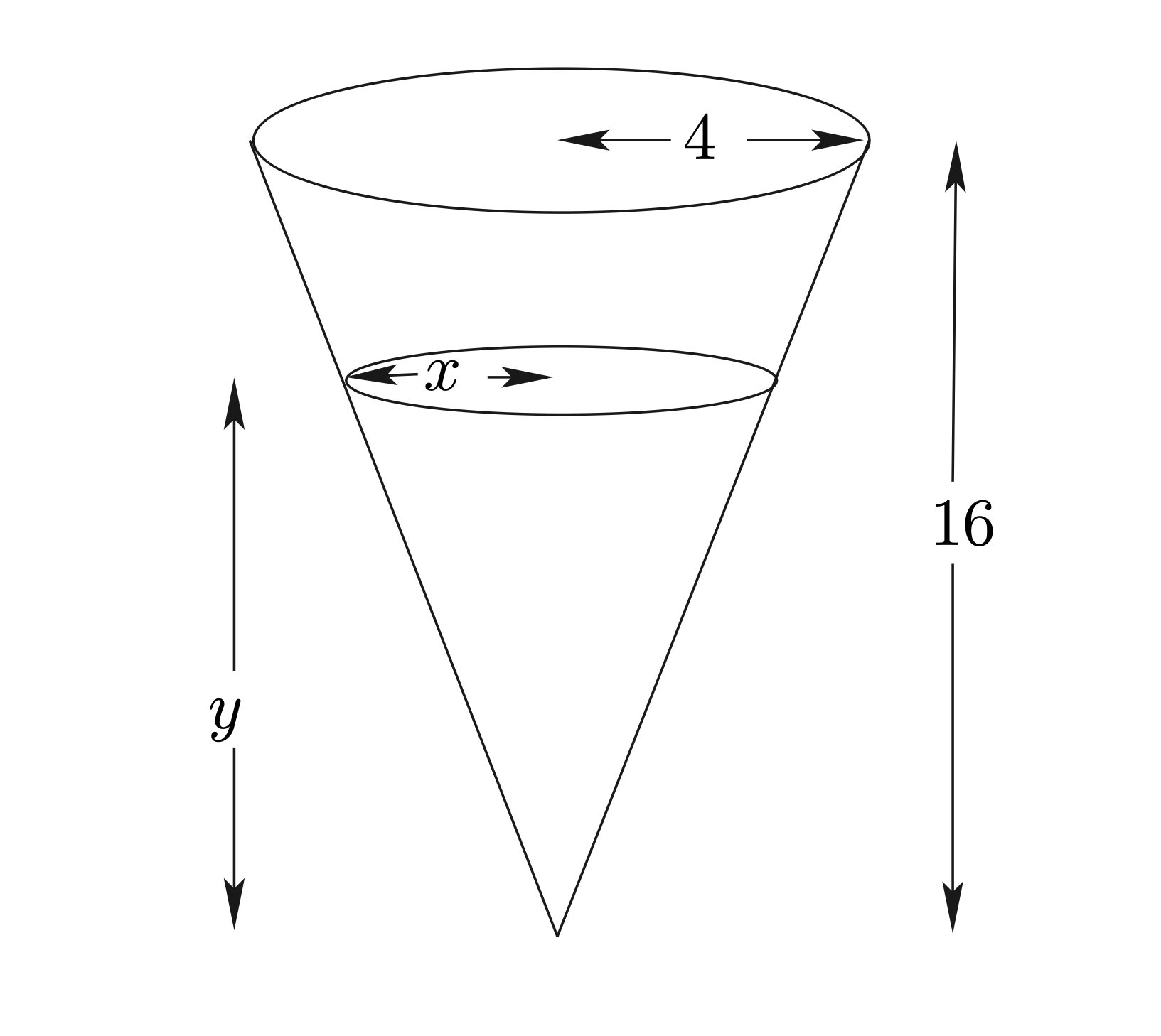
Figure 3.2: การไหลเวียนของอากาศในหลอดลม
กำหนดให้ \(t\) เป็นเวลานับจากการเริ่มต้นการสังเกต (min) \(V\) เป็นปริมาตรของน้ำในกรวย ณ เวลา \(t\) (in\(^3\)) \(y\) เป็นความลึกของน้ำในกรวย ณ เวลา \(t\) (in) \(x\) เป็นรัศมีของพื้นที่ผิวของน้ำ ณ เวลา \(t\) (in) อัตราการเปลี่ยนแปลงปริมาตรของน้ำ คือ \(\displaystyle \frac{dV}{dt}\) และ อัตราการเปลี่ยนแปลงความลึกของน้ำ คือ \(\displaystyle \frac{dy}{dt}\) โจทย์กล่าวว่าน้ำไหลออกจากกรวยด้วยอัตราเร็ว 2 in\(^3\)/min เมื่อระดับน้ำสูง 8 in แสดงว่า น้ำในกรวยมีปริมาตรลดลง \[\frac{dV}{dt}\bigg{|}_{y=8} = -2\] การระบุอัตราการเปลี่ยนแปลงแบบนี้ แสดงให้เห็นว่า ณ ความลึกของน้ำต่างกัน อัตราการเปลี่ยนแปลงปริมาตรของน้ำก็จะแตกต่างกันไป ไม่ได้เปลี่ยนแปลงด้วยอัตราที่คงที่เหมือนตัวอย่างก่อนหน้านี้ โจทย์ต้องการทราบว่าอัตราการเปลี่ยนแปลงความลึกของน้ำ เมื่อระดับน้ำสูง 8 นิ้ว นั่นคือ \(\displaystyle \frac{dy}{dt}\bigg{|}_{y=8}\)
จากสูตรการหาปริมาตรของกรวย \[V=\frac{1}{3}\pi x^2 y\] และจากคุณสมบัติของสามเหลี่ยมคล้าย \(\displaystyle \frac{x}{y}=\frac{4}{16}\) หรือ \(\displaystyle x=\frac{y}{4}\) ทำให้ได้ \(\displaystyle V=\frac{\pi}{48} y^3\) หาอนุพันธ์เทียบ \(t\) ทั้ง 2 ข้าง จะได้ \(\displaystyle \frac{dV}{dt}=\frac{\pi}{48} (3y^2 \frac{dy}{dt})\) หรือ \(\displaystyle \frac{dy}{dt}=\frac{16}{\pi y^2} \frac{dV}{dt}\) ดังนั้น \[\displaystyle \frac{dy}{dt}\bigg{|}_{y=8} = \frac{16(-2)}{\pi(8)^2} = \frac{-1}{2\pi} \text{ (in/min)}\] สรุปว่า เมื่อระดับน้ำสูง 8 นิ้ว ความลึกของน้ำจะลดลงด้วยอัตรา \(\displaystyle \frac{1}{2\pi}\) นิ้วต่อวินาที
ตัวอย่าง 3.26 เมื่อโยนก้อนหินลงในสระน้ำ จะเกิดคลื่นซึ่งรัศมีเพิ่มขึ้นด้วย อัตรา 0.9 เมตร/วินาที พื้นที่ที่ล้อมรอบไปด้วยคลื่นหลังจาก ผ่านไป 10 วินาทีเพิ่มขึ้นด้วยอัตราเท่าใด?
วิธีทำ กำหนดให้
\(t\) แทนเวลา (วินาที)
\(r\) แทนรัศมีของคลื่น (เมตร)
\(A\) แทนพื้นที่ที่ล้อมรอบไปด้วยคลื่น (ตารางเมตร)
พื้นที่ที่ล้อมรอบไปด้วยคลื่นเป็นไปตามสูตร \[A = \pi r^2\] เราหา derivative เทียบกับเวลา ได้ว่า \[\frac{dA}{dt} = 2\pi r\frac{dr}{dt}\] เรามีข้อมูลว่า \(\frac{dr}{dt} = 0.9\) เมตร ในขณะที่วินาที ที่ \(10\) รัศมีของคลื่นจึงมีค่าเท่ากับ \(0.9\cdot 10 = 9\) เมตร และดังนั้นพื้นที่ที่ล้อมรอบไปด้วยคลื่นจึงเพิ่มขึ้นด้วยอัตรา \[\frac{dA}{dt} = (2\pi)(9)(0.9) = 50.89\] ตารางเมตรต่อวินาที
ตัวอย่าง 3.27 เครื่องเททราย เททรายเป็นรูปกรวย ซึ่งความสูงของกองทรายมีค่าเท่ากับ เส้นผ่านศูนย์กลางที่ฐานของกองทรายเสมอ ถ้าความสูงเพิ่มขึ้นด้วยอัตราคงที่ 1.5 เมตร ต่อนาที จงหาว่าเครื่องเททรายเททรายด้วยอัตราเท่าใดเมื่อกองทรายมีความ สูงเท่ากับ 3 เมตร
วิธีทำ กำหนดให้
\(t\) แทนเวลา (นาที)
\(V\) แทนปริมาตรของกองทราย ณ เวลา \(t\) (ลูกบาศก์เมตร)
\(h\) แทนความสูงของกองทราย ณ เวลา \(t\) (เมตร)
\(r\) แทนรัศมีของพื้นกองทราย ณ เวลา \(t\) (เมตร)
ในแต่ละเวลา \(t\) อัตราการเปลี่ยนแปลงของปริมาตรทรายคือ \(dV/dt\) และอัตราการเปลี่ยนแปลงของความสูงของกองทรายคือ \(dh/dt\) จากข้อมูล ที่ให้มา เรารู้ว่า \[\frac{dh}{dt} = 1.5\] เนื่องจากกองทรายมีลักษณะเป็นรูปกรวย ซึ่งมีสูตรว่า \[V = \frac{1}{3}\pi r^2h\] เรายังทราบอีกว่า ที่แต่ละเวลา \(t\) ความสูงของกองทราย มีค่าเท่ากับรัศมีของพื้นกองทราย \(r=h\) เพราะฉะนั้น \[V = \frac{1}{3}\pi h^3\] หา derivative เทียบกับ \(t\) ได้ว่า \[\frac{dV}{dt} = \pi h^2\frac{dh}{dt}\] ดังนั้น \[\frac{dV}{dt} = 1.5\pi h^2\] เมื่อกองทรายสูง 3 เมตร อัตราการเปลี่ยนแปลงของปริมาตรกองทรายจึงเป็น \[\frac{dV}{dt} = 13.5\pi = 42.41\] ลูกบาศก์เมตรต่อนาที
ตัวอย่าง 3.28 จุด P เคลื่อนที่ไปตามเส้นโค้งตามสมการ \[y = \sqrt{x^2+16}\] เมื่อ \(P = (3,5)\) แล้ว \(y\) มีค่าเพิ่มขึ้นด้วยอัตรา 2 หน่วย/วินาที ค่า \(x\) มีการเปลี่ยนแปลงด้วยอัตราเท่าใด
วิธีทำ กำหนดให้
- \(t\) แทนเวลา (วินาที)
เราหา derivative ของสมการที่กำหนดเทียบกับเวลา \(t\) พบว่า \[\label{E:example} \frac{dy}{dt} = \frac{x}{\sqrt{x^2+16}}\frac{dx}{dt}\] เรารู้ว่าที่จุด \(P = (3,5)\) \[\frac{dy}{dt} = 2\] แทนค่าทั้งสองในสมการ \[E:example\] เราจะได้ว่า \[2 = \frac{2}{\sqrt{9+16}}\frac{dx}{dt}\] นั่นคือ \[\frac{dx}{dt} = 5\] นั่นคือ \(x\) มีการเปลี่ยนแปลงด้วยอัตรา 5 หน่วยต่อวินาที
ตัวอย่าง 3.29 ท่าเรือหนึ่ง มีแท่งแขวนลูกรอกผูกเรืออยู่เหนือท่า มีเชือกผูกไว้กับ หัวเรือซึ่งอยู่ต่ำกว่าตัวรอกของแท่งแขวน 3 เมตร ถ้าเราดึงเชือกด้วยอัตราเร็ว 6 เมตร/นาที เรือถูกดึงเข้าหาท่าด้วยอัตราเร็วเท่าใดเมื่อเชือก จากหัวเรือถึงลูกรอกมีความยาว 40 เมตร
วิธีทำ กำหนดให้
\(t\) แทนเวลา (นาที)
\(x\) ระยะทางในแนวนอน (เมตร)
\(y\) ระยะทางในแนวดิ่ง (เมตร)
จากข้อมูลของปัญหา เราสรูปได้ว่า อัตราการดึงเชือกแทนด้วยพจน์ \[\frac{dy}{dt} = 6\] คำถามให้ \(\frac{dx}{dt}\) เมื่อเชือกยาว 40 เมตรนับจากหัวเรือถึงลูกรอก โดยการใช้พิทาโกรัส เราจึงได้ความสัมพันธ์ \[x^2+y^2 = 40^2\] เราหา derivative เทียบกับ \(t\) ทั้งสองข้างของสมการ \[\begin{equation} \begin{aligned} 2x \frac{dx}{dt} + 2y\frac{dy}{dt} &= 0 \\ x \frac{dx}{dt} + y\frac{dy}{dt} &= 0 \end{aligned} \end{equation}\] เนื่องจากลูกรอกอยู่สูงกว่าหัวเรือ 3 เมตร หรือ \(y=3\) ในขณะที่ การดึงเชือกด้วยอัตราเร็ว 6 เมตร หรือ \(\frac{dy}{dt} = 6\) เพราะฉะนั้น เมื่อเชือกยาว 40 เมตร เรืออยู่ห่างออกไปเป็นระยะทาง \[x^2 + 3^2 = 40^2\] หรือ \(x = \sqrt{1591}\) ดังนั้น \[\begin{equation} \begin{aligned} \sqrt{1591}\frac{dx}{dt} + 4(6) &= 0 \\ \frac{dx}{dt} &= -\frac{24}{\sqrt{1591}} = -0.60 \end{aligned} \end{equation}\] ซึ่งหมายถึงเรือถูกดึงเข้าหาท่าด้วยอัตราเร็ว 0.6 เมตรต่อนาที
วาดภาพและกำหนดตัวแปรต่างๆ เช่น \(x\), \(y\) เป็นต้น
ระบุอัตราการเปลี่ยนแปลงของตัวแปรทุกตัวที่โจทย์กำหนดให้ และที่โจทย์ต้องการให้หา เช่น \(\displaystyle\frac{dx}{dt}\), \(\displaystyle\frac{dy}{dt}\) เป็นต้น
หาสมการสมการหนึ่งที่แสดงให้เห็นถึงความสัมพันธ์ระหว่างตัวแปรที่กำหนดขึ้นในขั้นตอนที่ 1 และเมื่อหาอนุพันธ์ของสมการนี้ จะมีเทอมที่เกี่ยวข้องกับอนุพันธ์ในขั้นตอนที่ 2
หาอนุพันธ์ทั้ง 2 ข้างของสมการในขั้นตอนที่ 3 เทียบกับเวลาและนำค่าของอนุพันธ์ที่ทราบลงไปในสมการ
หาค่าของอนุพันธ์ที่โจทย์ต้องการด้วยวิธีทางพีชคณิต
3.8.4 แบบฝึกหัด
กำหนดให้ \(y= \ln x\) จงหา \(dy\) และ \(\Delta y\) ที่ \(x=1\) โดย ที่ \(dx = \Delta x = 0.5\)
พิจารณาฟังก์ชันต่อไปนี้ แล้วหาสูตร \(dy\) และ \(\Delta y\)
\(\displaystyle y = x\sqrt{x-1}\)
\(\displaystyle y = xe^x\)
\(\displaystyle y = x\sin x\)
\(\displaystyle y = \tan (x^2)\)
จงหา local linear approximation ของเส้นโค้งจากสมการ \(xe^y = y\) ที่จุด \((0,0)\) และใช้สมการที่ได้ประมาณค่าของ \(y\) เมื่อ \(x=0.1\)
จงหา \(\frac{dy}{dx}\) สำหรับความสัมพันธ์ต่อไปนี้
\(x^2+ y^2 = 25\)
\(\frac{1}{x} + \frac{1}{y} = 1\)
\(x\sin y + y\sin x = 1\)
\(e^{xy} + xy = 1\)
หญิงคนหนึ่งสูง 1.55 เมตร เดินเข้าเสาไฟด้วยอัตราเร็ว 0.75 เมตร/วินาที เสาไฟติดดวงไฟสูง 5 เมตร
เงาของหญิงคนนี้เปลี่ยนแปลงด้วยอัตราเท่าใด
ปลายเงาของด้านศรีษะหญิงคนนี้เคลื่อนที่ด้วยอัตราเร็วเท่าใด
อนุภาคหนึ่งเคลื่อนที่ไปตามเส้นโค้งอธิบายตามสมการ \[\frac{x^2y}{1+y^2} = \frac{2}{5}\] กำหนดให้พิกัดแกน \(x\) ของอนุภาคเพิ่มขึ้นด้วยอัตรา 4 หน่วย/วินาที เมื่ออนุภาคอยู่ที่ตำแหน่ง \((1,2)\)
พิกัดแกน \(y\) ของอนุภาคเปลี่ยนแปลงด้วยอัตราเท่าใด เมื่ออนุภาคอยู่ที่ตำแหน่ง \((1,2)\)
ณ ตำแหน่ง \((1,2)\) อนุภาคกำลังเคลื่อนสูงขึ้นหรือลดลงในพิกัด \(xy\)
ความเข้มของแสงที่ผ่านเข้าตาขึ้นอยู่กับรัศมีของ pupil ถ้า pupil มีขนาดมากขึ้น ปริมาณของแสงก็จะเข้าตามากขึ้น ดังสมการ \(I=kr^2\) เมื่อ \(I\) เป็นความเข้มของแสง \(r\) เป็นรัศมีของ pupil และ \(k\) เป็นค่าคงตัว ในช่วงเวลา 6 โมงเช้าถึงเที่ยง รัศมีของ pupil จะขยายตัวด้วยอัตราเร็วคงที่ 0.1 mm/min จงหาว่าในช่วงเวลาดังกล่าว ความเข้มของแสงที่ผ่านเข้าตา จะมีการเปลี่ยนแปลงอย่างไร เมื่อ \(r=0.5\) cm
การแพร่ระบาดของแมลงวันทอง เริ่มที่ใจกลางของหมู่บ้านเล็กๆ แห่งหนึ่งนอกเมือง พื้นที่การแพร่ระบาดมีลักษณะคล้ายวงกลมดังแสดงในรูป 1.5 รัศมีของพื้นที่การแพร่ระบาดขยายเพิ่มขึ้นด้วยอัตรา 1.5 ไมล์ต่อปี จงหาอัตราการเปลี่ยนแปลงของพื้นที่การแพร่ระบาด เมื่อรัศมีของพื้นที่การแพร่บาดมีค่าเท่ากับ 4 ไมล์
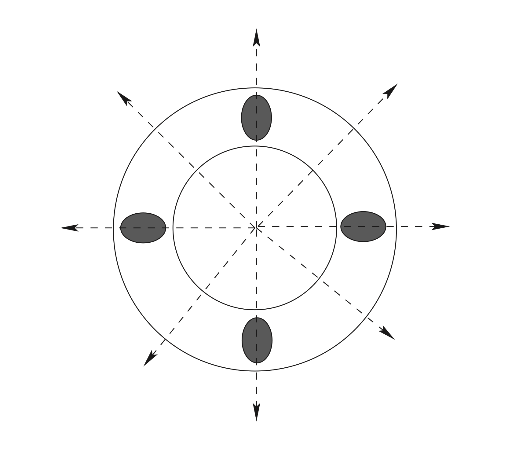
Figure 3.3: การแพร่ระบาดของแมลงวันทอง โดยที่วงรีสีเทาแทนแมลงวัน
3.9 อนุพันธ์ของฟังก์ชันตรีโกณมิติและอินเวอร์สของฟังก์ชันตรีโกณมิติ
3.9.1 อนุพันธ์ของฟังก์ชันตรีโกณมิติ
เราจะใช้ความรู้เกี่ยวกับเอกลักษณ์ตรีโกณมิติและลิมิตของฟังก์ชันตรีโกณ
ช่วยในการหาอนุพันธ์ของฟังก์ชันตรีโกณมิติโดยนิยามดังนี้
\[\begin{equation} \begin{aligned}
\lim_{x\rightarrow 0} \frac{\sin x}{x} &= 1 \quad \text{ เมื่อ x มีหน่วยเป็นเรเดียน }\\
\lim_{x\rightarrow 0} \frac{\cos x -1}{x} &= 1 \\
\sin A- \sin B &=2 \cos \frac{A+B}{2}\sin \frac{A-B}{2}
\end{aligned} \end{equation}\]
ทฤษฎี 3.4 ถ้า \(f(x)=\sin x\) แล้ว \(\displaystyle \frac{d}{dx}\sin x =\cos x\)
\[\begin{equation} \begin{aligned} \displaystyle \frac{d}{dx}\sin x&=\lim_{h\rightarrow 0}(\frac{\sin (x+h)-\sin x}{h})\\ \displaystyle &=\lim_{h\rightarrow0} \frac{2\cos (x+\frac{h}{2})\sin \frac{h}{2}}{h}\\ \displaystyle &=2\lim_{h\rightarrow 0}\cos (x+\frac{h}{2}).\lim_{h\rightarrow 0} \frac{\sin \frac{h}{2}}{h}\\ \displaystyle &=2\cos x\lim_{\frac{h}{2} \rightarrow 0}\frac{\frac{1}{2}\sin \frac{h}{2}}{\frac{h}{2}}\\ \displaystyle &=2(\cos x)\frac{1}{2}\\ &=\cos x \end{aligned} \end{equation}\]
เนื่องจาก \[\begin{equation} \begin{aligned} \sin (x+h)- \sin x &=2\cos \frac{x+h+x}{2}\sin \frac{h}{2}\\ &=2\cos (x+\frac{h}{2})\sin \frac{h}{2} \end{aligned} \end{equation}\]
สำหรับการหาอนุพันธ์ของ cosine ก็ทำได้ในทำนองเดียวกันกับ sine ส่วนฟังก์ชันตรีโกณมิติอื่นๆ
หาได้โดยแปลงในรูป cosine หรือ sine เช่น
\[\tan x= \frac{\sin x}{\cos x}, \quad \cot x=\frac{\cos x}{\sin x}, \quad \sec x=\frac{1}{\cos x} \text{ และ } \displaystyle \csc x=\frac{1}{\sin x}\]
ทฤษฎี 3.5
\(\displaystyle\frac{d}{dx}\cos x=-\sin x\)
\(\displaystyle\frac{d}{dx}\tan x=\sec^{2} x\)
\(\displaystyle\frac{d}{dx}\cot x=-\csc^{2} x\)
\(\displaystyle\frac{d}{dx}\sec x=\sec x \tan x\)
\(\displaystyle\frac{d}{dx}\csc x=-\csc x\cot x\)
\[\begin{equation} \begin{aligned} \displaystyle \frac{d}{dx}\sec x&=\frac{d}{dx}.\frac{1}{\cos x}\\ &=\frac{d}{dx}(\cos x)^{-1}\\ &=(-1)(\cos x)^{-2}\displaystyle \frac{d}{dx}\cos x\\ &=\displaystyle \frac{-1}{\cos^{2} x}(-\sin x)\\ &=\displaystyle \frac{1}{\cos x}.\frac{\sin x}{\cos x}\\ &=\sec x\tan x \end{aligned} \end{equation}\]
ตัวอย่าง 3.30 กำหนดให้ \(y=x^{2}\tan 3x\) จงหา \(\displaystyle \frac{dy}{dx}\)
วิธีทำ \[\begin{equation} \begin{aligned} \displaystyle \frac{dy}{dx}&=\frac{d}{dx}(x^{3}\tan 3x)\\ &=x^{2}\displaystyle \frac{d}{dx}\tan 3x+\tan 3x\frac{d}{dx}x^{2}\\ &=x^{2}(\sec^{2}3x)(3)+(\tan 3x)(2x)\\ &=3x^{2}\sec^{2}3x+2x\tan 3x \end{aligned} \end{equation}\]
ตัวอย่าง 3.31 กำหนดให้ \(\displaystyle y=\frac{\sin x}{1+\cos x}\) จงหา \(\displaystyle \frac{dy}{dx}\)
วิธีทำ \[\begin{equation} \begin{aligned} \displaystyle \frac{dy}{dx}&=\frac{d}{dx}(\frac{\sin x}{1+\cos x})\\ &=\frac{(1+\cos x)\displaystyle \frac{d}{dx}\sin x -\sin x\displaystyle \frac{d}{dx}(1+\cos x)}{(1+\cos x)^{2}}\\ &=\frac{(1+\cos x)\cos x-(\sin x)(-\sin x)}{(1+\cos x)^{2}}\\ &=\frac{\cos x+\cos^{2}x+\sin^{2}x }{(1+\cos x)^{2}}\\ &=\frac{\cos x+1}{(1+\cos x)^{2}}\\ &=\frac{1}{1+\cos x} \end{aligned} \end{equation}\]
ตัวอย่าง 3.32 กำหนดให้ \(y=\sec^{2}(3x-1)\) จงหา \(\displaystyle \frac{dy}{dx}\)
วิธีทำ \[\begin{equation} \begin{aligned} \displaystyle \frac{dy}{dx}&=\frac{d}{dx}\sec^{2}(3x-1)\\ &=2\sec(3x-1)\displaystyle \frac{d}{dx}\sec(3x-1)\\ &=2\sec(3x-1)\sec(3x-1)\tan(3x-1)\displaystyle \frac{d}{dx}(3x-1)\\ &=3.2\sec^{2}(3x-1)\tan(3x-1)\\ &=6\sec^{2}(3x-1)\tan(3x-1) \end{aligned} \end{equation}\]
ตัวอย่าง 3.33 ถ้า \(x\cos y+y\cos x=1\) จงหา \(\displaystyle \frac{dy}{dx}\)
วิธีทำ ใช้ implicit differentiation \[\begin{equation} \begin{aligned} \displaystyle \frac{d}{dx}(x\cos y +y\cos x)&=\frac{d}{dx}1\\ \displaystyle \frac{d}{dx}(x\cos y)+\frac{d}{dx}(y\cos x)&=0\\ \displaystyle x\frac{d}{dx}\cos y+\cos y \frac{dx}{dy}+y\frac{d}{dx}\cos x+\cos x\frac{dy}{dx}&=0\\ \displaystyle x(-\sin y)\frac{dy}{dx}+\cos y + y(-\sin x)+\cos x\frac{dy}{dx}&=0\\ \displaystyle (-x\sin y+\cos x)\frac{dy}{dx}&=y\sin x -\cos y\\ \displaystyle \frac{dy}{dx}&=\frac{y\sin x-\cos y}{\cos x-x\sin y} \end{aligned} \end{equation}\]
ตัวอย่าง 3.34 จงหา \(\displaystyle \frac{d^{2}y}{dx^{2}}\) ของฟังก์ชัน \(y= x\cos x\)
วิธีทำ \[\begin{equation} \begin{aligned} y&= x\cos x\\ \displaystyle y'&=\frac{d}{dx}(x\cos x)\\ &=\displaystyle \frac{d}{dx}\cos x +\cos x\frac{dx}{dx}\\ &=-x\sin x + \cos x\\ \displaystyle y''&=-(x\frac{d}{dx}\sin x + \sin x\frac{dx}{dx}) + \frac{d}{dx}\cos x \\ &=-(x\cos x + \sin x)-\sin x\\ &=-x\cos x - 2\sin x \end{aligned} \end{equation}\]
3.9.2 อนุพันธ์ของฟังก์ชันอินเวอร์สของฟังก์ชันตรีโกณมิติ
จะเห็นว่าฟังก์ชันตรีโกณมิติทั้งหมดคือ sine, cosine, tangent, cotangent, secant และ cosecant เป็นฟังก์ชันคาบซึ่งสมาชิกในโดเมน จะให้ค่าซ้ำกัน ดังนั้น ฟังก์ชันตรีโกณมิติจึงไม่เป็น 1-1 ฟังก์ชัน แต่เราสามารถจำกัดโดเมนของฟังก์ชันตรีโกณมิติเพื่อทำให้ฟังก์ชันเหล่านี้ เป็น 1-1 ฟังก์ชัน ก็จะทำให้อินเวอร์สของฟังก์ชันเหล่านั้นเป้นฟังก์ชันด้วย เช่น \[F=\{(x,y)|y=\sin x\} \text{ มีโดเมน }=\Re \text { และเรนจ์ }=[-1,1]\] ไม่เป็น1-1ฟังก์ชัน แต่ \[F=\{(x,y)|y=\sin x , x\in \displaystyle [-\frac{\pi}{2},\frac{\pi}{2}]\}\] เป็น 1-1 ฟังก์ชัน ดังนั้น \[F^{-1}=\{(x,y)|x=\sin y , y\in \displaystyle [-\frac{\pi}{2},\frac{\pi}{2}], x\in [-1,1]\}\] เป็น อินเวอร์สฟังก์ชันของ\(F\)เรียกว่า inverse sine function ใช้สัญลักษณ์ \(\sin^{-1} x\) หรือ \(\arcsin x\)
ในทำนองเดียวกัน
ทฤษฎี 3.6
\(\displaystyle\frac{d}{dx} \arcsin x=\frac{1}{\sqrt{1-x^{2}}}., |x|<1\)
\(\displaystyle\frac{d}{dx} \arccos x=\frac{-1}{\sqrt{1-x^{2}}}., |x|<1\)
\(\displaystyle\frac{d}{dx} arccot x=\frac{-1}{1+x^{2}}.\)
\(\displaystyle\frac{d}{dx} arcsec x=\frac{1}{|x|\sqrt{x^{2}-1}}, |x|>1\)
\(\displaystyle\frac{d}{dx} arccosec x=\frac{-1}{|x|\sqrt{x^{2}-1}}, |x|>1\)
\(\displaystyle\frac{d}{dx} \arctan x=\frac{1}{1+x^{2}}\)
ให้ \(y=\arcsin x , |x|<1\)
\[\begin{equation} \begin{aligned}
x&=\sin y, \displaystyle \frac{-\pi}{2}\leq y \leq \frac{\pi}{2}\\
\displaystyle \frac{dx}{dx}&=\frac{d}{dx}\sin y\\
1&=\cos y \displaystyle \frac{dy}{dx}\\
\displaystyle \frac{dy}{dx}&=\frac{1}{\cos y} , |x|<1\\
&=\displaystyle \frac{1}{\sqrt{1-\sin^{2} y}}\\
&=\displaystyle \frac{1}{\sqrt{1-x^{2}}}
\end{aligned} \end{equation}\]
ตัวอย่าง 3.35 จงหา \(\displaystyle \frac{dy}{dx}\) เมื่อ \(y=\sin^{-1}(2x)\)
วิธีทำ \[\begin{equation} \begin{aligned} \displaystyle \frac{dy}{dx}&=\frac{1}{\sqrt{1-(2x)^{2}}}.\frac{d}{dx}(2x)\\ &=\frac{2}{\sqrt{1-4x^{2}}} \end{aligned} \end{equation}\]
ตัวอย่าง 3.36 จงหา \(y'\) เมื่อ \(y=arcsec x^{2}\)
วิธีทำ \[\begin{equation} \begin{aligned} \displaystyle y'&=\frac{d}{dx}arcsec x^{2}\\ &=\displaystyle \frac{1}{|x|^{2}\sqrt{x^{4}-1}}.\frac{d}{dx}(x)^{2}\\ &=\displaystyle \frac{2x}{x^{2}\sqrt{x^{4}-1}}\\ &=\displaystyle \frac{2}{x\sqrt{x^{4}-1}} \end{aligned} \end{equation}\]
ตัวอย่าง 3.37 จงหา \(y'\) เมื่อ \(y=cot^{-1}\displaystyle(\frac{1}{x})-\tan^{-1}x\)
วิธีทำ \[\begin{equation} \begin{aligned} \displaystyle y&=\cot^{-1}(\frac{1}{x})-\tan^{-1}\\ \displaystyle y'&=\frac{d}{dx}(\cot^{-1}(\frac{1}{x})-\tan^{-1})\\ \displaystyle &=\frac{d}{dx}\cot^{-1}(\displaystyle \frac{1}{x})-\frac{d}{dx}\tan^{-1}x\\ \displaystyle &=\frac{-1}{1-\displaystyle \frac{1}{x^{2}}}(-\frac{1}{x^{2}})-\frac{1}{1+x^{2}}\\ \displaystyle &=\frac{1}{x^{2}-1}-\frac{1}{1+x^{2}}\\ \displaystyle &=\frac{2}{x^{4}-1} \end{aligned} \end{equation}\]
3.10 อนุพันธ์ของฟังก์ชันเอกซ์โพเนนเชียลและฟังก์ชันลอการิทึม
ในบทที่ 1 เราอธิบายการขยายพันธ์แบคทีเรีย \(N(t)\) ในรูปของเวลา \(t\) ในรูปของแบบจำลองทางคณิตศาสตร์ โดยมีสมการดังต่อไปนี้
\[\begin{align} \frac{N(t + h) - N(t)}{h} &= b\cdot N(t) - m\cdot N(t)\\ \tag{3.1} \end{align}\]
ในทางคณิตศาสตร์เราเรียกสมการดังกล่าวว่า สมการเชิงอนุพันธ์สามัญ (ordinary differential equation) และมีเนื้อหาในรายวิชานี้ที่จะเรียนในบทถัดๆ ไป ทั้งนี้ฟังก์ชัน \(N(t)\) ที่ปรากฏในสมการเป็นฟังก์ชันไม่ทราบค่า (unknown function) และเราสามารถหาคำตอบของสมการเชิงอนุพันธ์ที่มีเงื่อนไขเริ่มต้นโดยวิธีการหาปริพันธ์ (Integration) ได้คำตอบของสมการดังนี้
\[\begin{equation} N(t) = N_0 e^{(b-m)t} \tag{3.2} \end{equation}\]
ดังนั้นในบทนี้ เราจะกล่าวถึงอนุพันธ์ของฟังก์ชันเอกซ์โพเนนเชียลและฟังก์ชันลอการิทึม เราสามารถใช้นิยาม หรือสูตรต่อไปนี้ในการหาอนุพันธ์
ทฤษฎี 3.7
- \(\displaystyle\frac{d}{dx}e^x = e^x\)
- \(\displaystyle\frac{d}{dx}a^x = a^x \ln a \quad (a > 0, a \neq 1)\)
- \(\displaystyle\frac{d}{dx}\ln x = \frac{1}{x}\)
- \(\displaystyle\frac{d}{dx}\log_a x = \frac{1}{x \ln a} \quad (a > 0, a \neq 1)\)
ตัวอย่าง 3.38 จงหาอนุพันธ์ของ \(f(x) = e^{x^2 + 1}\)
วิธีทำ
เราสามารถใช้กฏลูกโซ่ในการหาอนุพันธ์ของ \(f(x) = e^{x^2 + 1}\) ได้ดังต่อไปนี้
โดยการกำหนดให้ \(u = x^2 + 1\), แล้ว \(f(x) = e^u\) และจะได้ว่า
\[ \frac{d}{dx} f(x) = \frac{d}{du} e^u \cdot \frac{d}{dx} u \]
เนื่องจาก \(\frac{d}{du} e^u = e^u\) และ \(\frac{d}{dx} u = \frac{d}{dx} (x^2 + 1) = 2x\).
ดังนั้น
\[ \frac{d}{dx} f(x) = e^u \cdot 2x \]
เมื่อแทนตัวแปร \(u = x^2 + 1\) ลงในสมการข้างต้น เราจะได้ว่า
\[ \frac{d}{dx} f(x) = e^{x^2 + 1} \cdot 2x \]
ดังนั้น อนุพันธ์ของ \(f(x) = e^{x^2 + 1}\) คือ
\[ \boxed{\frac{d}{dx} f(x) = 2x e^{x^2 + 1}} \]
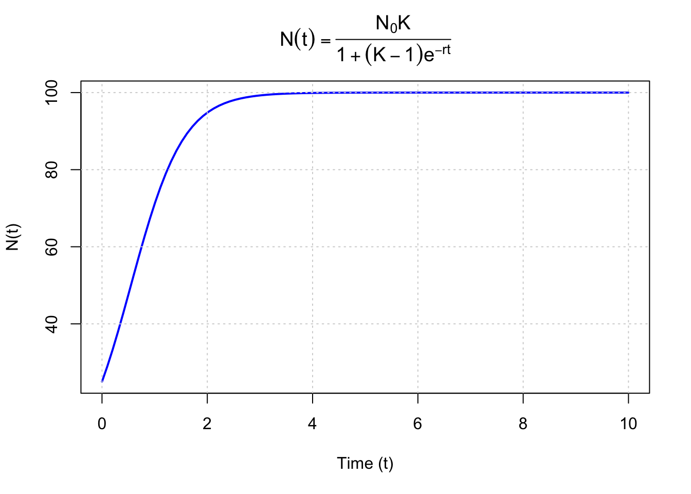
ตัวอย่าง 3.39 จงแสดงว่า \(N(t) = \frac{K}{1 + (K - 1) e^{-rt}}\) เป็นคำตอบของสมการเชิงอนุพันธ์
\[ \frac{dN}{dt} = rN\left(1 - \frac{N}{K}\right) \]โดยที่ \(r\) และ \(K\) เป็นค่าคงตัวที่เป็นบวก สมการเชิงอนุพันธ์นี้มีชื่อเรียกว่า the logistic growth equation
วิธีทำ
หาอนุพันธ์ของฟังก์ชัน \(N(t)\):
กำหนดให้ \(N(t) = \frac{K}{1 + (K - 1) e^{-rt}}\).
เราสามารถใช้กฏลูกโซ่ในการหาอนุพันธ์ได้ผลลัพธ์ดังต่อไปนี้
\[ \frac{dN}{dt} = -\frac{K \cdot (K - 1) \cdot (-r) e^{-rt}}{(1 + (K - 1) e^{-rt})^2} \]
จัดรูปสมการให้อยู่ในรูปอย่างง่าย
\[ \frac{dN}{dt} = \frac{rK(K - 1) e^{-rt}}{(1 + (K - 1) e^{-rt})^2} \]
แทน \(N(t)\) ลงใน the logistic equation:
เนื่องจาก\[ \frac{dN}{dt} = rN\left(1 - \frac{N}{K}\right) \]
โดยการแทน \(N(t) = \frac{K}{1 + (K - 1) e^{-rt}}\) ลงไปในสมการข้างต้น เราจะได้ว่า
\[ rN\left(1 - \frac{N}{K}\right) = \frac{rK(K - 1) e^{-rt}}{(1 + (K - 1) e^{-rt})^2} \]
ผลสรุปที่ได้จากการหาอนุพันธ์ และการแทนค่าฟังก์ชัน
เราจะเห็นว่าทั้ง 2 ข้างของสมการข้างต้นเท่ากัน แสดงว่า ฟังก์ชัน \(N(t) = \frac{K}{1 + (K - 1) e^{-rt}}\) เป็นคำตอบของสมการ the logistic growth equation
หมายเหตุ จากตัวอย่างข้างต้นเราสมมติให้ \(N(0) = 1\) ในกรณีที่กำหนดให้ \(N(0) = N_0\) แล้วคำตอบของสมการ the logistic growth equation จะอยู่ในรูป
\[N(t) = \frac{N_0 \cdot K}{1 + (K - 1) e^{-rt}}\]
รูปต่อไปนี้แสดงกราฟของคำตอบของแบบจำลองการเติบโตแบบ logistic เมื่อกำหนดให้ \(N_0 = 25\), \(K = 4\) และ \(r = 2\) กราฟจะมีลักษณะเป็นรูปตัว \(S\) (ซิกมอยด์, sigmoidal) ซึ่งสะท้อนการเติบโตที่จำกัดเนื่องจากความจุที่รองรับได้ (carrying capacity) หรือค่า K ในตอนแรก ประชากรจะเติบโตแบบเอ็กซ์โพเนนเชียล แต่เมื่อเข้าใกล้ \(K\) อัตราการเติบโตจะช้าลงและกราฟจะแบนลง ซึ่งแตกต่างจากแบบจำลองการเติบโตแบบเอ็กซ์โพเนนเชียลธรรมดา โดยประชากรจะเติบโตโดยไม่มีขอบเขต โดยเป็นไปตามกราฟที่เพิ่มขึ้นอย่างต่อเนื่อง ในโมเดลโลจิสติกส์ การเติบโตถูกจำกัดและจะคงตัวเมื่อจำนวนประชากรใกล้ถึงขีดจำกัดความจุ
ตัวอย่าง 3.40 จงหาอนุพันธ์ของฟังก์ชัน:
\[ y = \frac{e^x \cdot x^2}{\sqrt{x^2 + 1}} \]
โดยใช้การลอการิทึมทั้งสองฝั่งก่อนทำการหาอนุพันธ์
วิธีทำ
ลอการิทึมทั้งสองข้าง:
\[ \ln y = \ln\left( \frac{e^x \cdot x^2}{\sqrt{x^2 + 1}} \right) \]
ใช้สมบัติลอการิทึม
\[ \ln y = \ln(e^x) + \ln(x^2) - \frac{1}{2} \ln(x^2 + 1) \]
ย่อ:
\[ \ln y = x + 2 \ln x - \frac{1}{2} \ln(x^2 + 1) \]
หาอนุพันธ์ทั้งสองข้าง:
\[ \frac{1}{y} \frac{dy}{dx} = 1 + \frac{2}{x} - \frac{1}{2} \cdot \frac{2x}{x^2 + 1} \]
ย่อ:
\[ \frac{1}{y} \frac{dy}{dx} = 1 + \frac{2}{x} - \frac{x}{x^2 + 1} \]
จัดรูปหา \(\frac{dy}{dx}\):
\[ \frac{dy}{dx} = y \left( 1 + \frac{2}{x} - \frac{x}{x^2 + 1} \right) \]
แทนค่า \(y = \frac{e^x \cdot x^2}{\sqrt{x^2 + 1}}\):
\[ \frac{dy}{dx} = \frac{e^x \cdot x^2}{\sqrt{x^2 + 1}} \left( 1 + \frac{2}{x} - \frac{x}{x^2 + 1} \right) \]
ดังนั้น อนุพันธ์ของ \(y = \frac{e^x \cdot x^2}{\sqrt{x^2 + 1}}\) คือ:
\[ \boxed{\frac{dy}{dx} = \frac{e^x \cdot x^2}{\sqrt{x^2 + 1}} \left( 1 + \frac{2}{x} - \frac{x}{x^2 + 1} \right)} \]