Chapter 5 Poisson processes

5.1 Introduction

In this chapter, we will consider a class of stochastic processes, namely Poisson processes, that can be used to model the occurrence or arrival of events over a continuous time interval. Time domains of such processes are continuous and the state space is the set of whole numbers.

For instance, consider the number of claims that occur up to time $t$ (denoted by $N(t) = N_t$) from a portfolio of health insurance policies (or other types of insurance products). Suppose that the average rate of occurrence of claims per time unit (e.g. day or week ) is given by $\lambda$.

Here are some questions of interest:

Suppose that on average 20 claims arrive every day (i.e. $\lambda = 20$). What is the probability that more than 100 claims arrive within a week?
What is the expected time until the next claim?

The model used to model the insurance claims is an example of Poisson processes. The following examples can also be modelled by a Poisson process:

Claims arrivals at an insurance company,
Telephone calls to a call center,
Accidents occurring on the highway.

5.2 Poisson process

A Poisson process is a special type of counting process. It can be represented by a continuous time stochastic process $\{N(t)\}_{t \ge 0}$ which takes values in the non-negative integers. The state space is discrete but the time set is continuous. Here $N(t)$ represents the number of events in the interval $(0,t]$.

5.2.1 Counting Process

A counting process $\{N(t)\}_{t \ge 0}$ is a collection of non-negative, integer-valued random variables such that if $0 \le s \le t$, then $N(s) \le N(t)$.

Figure 5.1 illustrates a trajectory of the Poisson process. An R code to simulate the trajectory is also given below. The sample path of a Poisson process is a right-continuous step function. There are jumps occurring at time $t_1, t_2, t_3, \ldots$.

lambda <- 17
# the length of time horizon for the simulation T_length <- 31
last_arrival <- 0
arrival_time <- c()
inter_arrival <- rexp(1, rate = lambda)
T_length <- 1
while (inter_arrival + last_arrival < T_length) { 
  last_arrival <- inter_arrival + last_arrival 
  arrival_time <- c(arrival_time,last_arrival) 
  inter_arrival <- rexp(1, rate = lambda)
}


n <- length(arrival_time)
counts <- 1:n

plot(arrival_time, counts, pch=16, ylim=c(0, n))
points(arrival_time, c(0, counts[-n]))
segments(
  x0 = c(0, arrival_time[-n]),
  y0 = c(0, counts[-n]),
  x1 = arrival_time,
  y1 = c(0, counts[-n])
)

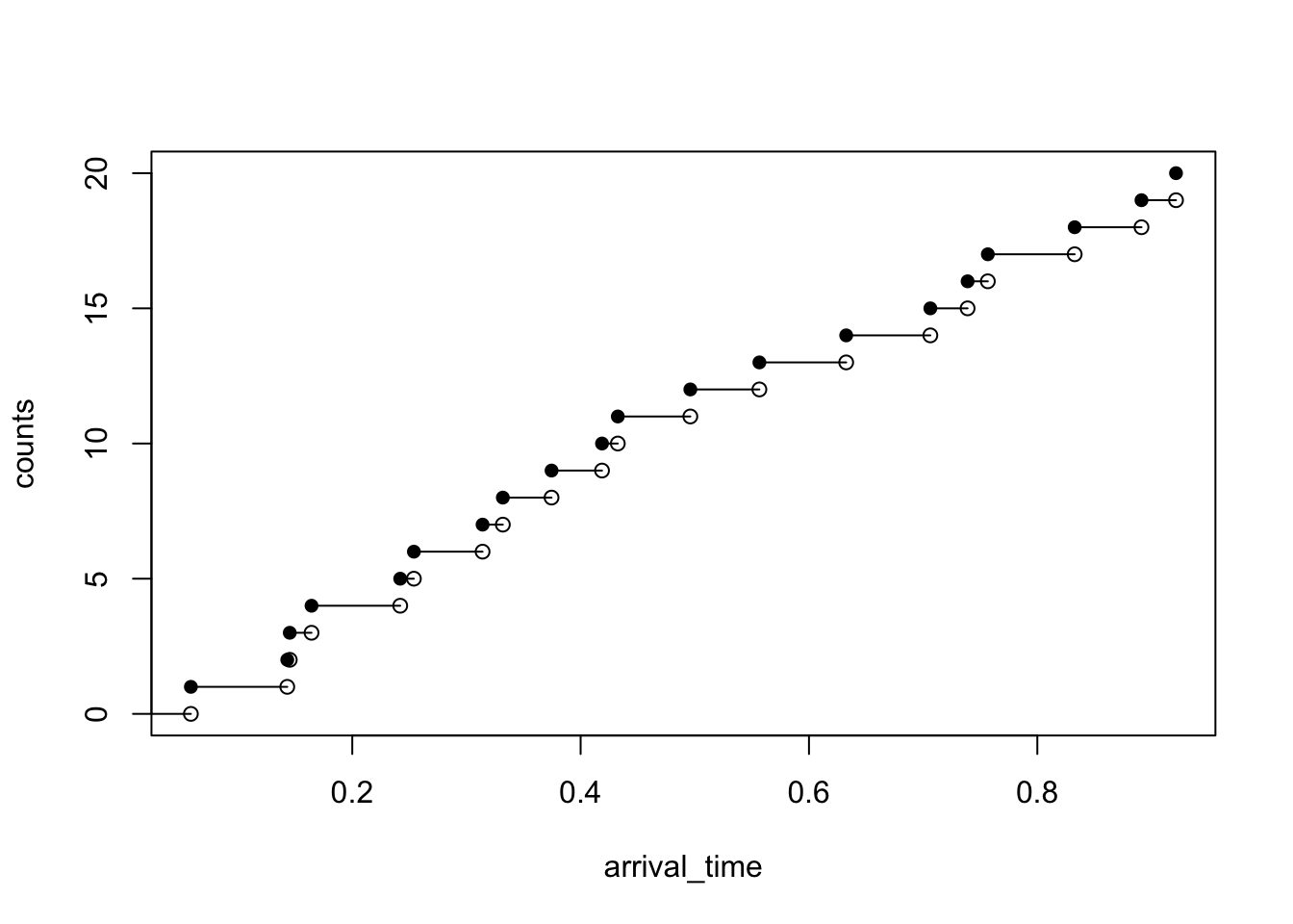
Figure 5.1: A trajectory of the Poisson process

We will see that there are several ways to describe a Poisson process. One can define it by the number of claims that occur up to time $t$ or the times between those claims when they occur. Main properties of Poisson processes will be discussed.

For $0 \le s < t$, the number of events in the interval $(s, t]$ is given by \[N(s,t) = N(t) - N(s).\] For any interval $I = (s,t]$, \[N(I) = N(t) - N(s).\] Therefore, $N(t) = N(0,t)$.

Formally, an integer-valued process $\{N(t)\}_{t \ge 0}$ is a Poisson process with rate $\lambda$ (or intensity) if it satisfies the following two conditions:

For any $t$ and $h> 0$ ($h$ small), \[\begin{aligned} \Pr(N(t+h) - N(t) = 1) &= \lambda h + o(h)\\ \Pr(N(t+h) - N(t) = 0) &= 1- \lambda h + o(h)\\ \Pr(N(t+h) - N(t) \ge 2) &= o(h) \end{aligned}\]
For disjoint intervals $I_1, I_2, \ldots, I_k$, the number of events $N(I_1), \ldots, N(I_k)$ are independent random variables.

Notes The statement that $f(h) = o(h)$ as $h \rightarrow 0$ means $\displaystyle\lim_{h\rightarrow 0} \frac{f(h)}{h} = 0$. Examples are $h^2$, $h^3$, etc.

The probability that an event occurs during the short time interval from time $t$ to time $t + h$ is approximately equal to $\lambda \, h$ for small $h$, i.e. \[\Pr[N(t+h) - N(t) = 1] \approx \lambda\, h.\] The parameter $\lambda$ represents the average rate of occurrence of events (e.g. 20 claims (or events) per day).
The properties essentially require that, in a very small interval of length $h$, we have either a single point (or an occurrence) with probability $\lambda h$, or no point with probability $1 - \lambda h$.
Any two of the three statements necessarily imply the third (since the sum of the probability of all possible outcomes is 1).

5.3 Properties of Poisson processes

In the following example, we show that $N(t)$ is a Poisson random variable with mean $\lambda t$ . In addition, $N(t +s) - N(s)$ is a Poisson random variable with mean $\lambda \, t$ , independent of anything that has occurred before time $s$.

Example 5.1 Show that the process $N(t)$ is a Poisson random variable with mean $\lambda t$, i.e. $N(t) \sim \text{Poisson}(\lambda \, t)$.

Solution:

To show that $N(t) \sim \text{Poisson}(\lambda t)$, we let \[p_j(t) = \Pr(N(t) = j),\] which is the probability that there have been exactly $j$ events by time $t$.

We simply need to show that \[ p_j(t) = \frac{e^{-\lambda t}(\lambda t)^j}{j!}\]

Case 1: For any $j >0$ and for small positive $h$, consider the following arguments

\[ \begin{aligned} p_j(t+h) &= \Pr(N(t+h) = j) \\ &= \Pr(N(t) = j \text{ and } N(t,t+h) = 0) \\ &+ \Pr(N(t) = j-1 \text{ and } N(t,t+h) = 1) \\ &+ \Pr(N(t) < j-1 \text{ and } N(t,t+h) \ge 2) \\ &= p_j(t)(1 - \lambda h) + p_{j-1}(t)(\lambda h) + o(h) \end{aligned} \] Rearranging the equation and dividing both sides of the equation by $h$ yields \[ \begin{aligned} \frac{p_j(t+h) - p_j(t)}{h} &= \lambda p_j(t) + \lambda p_{j-1}(t) + \frac{o(h)}{h}. \end{aligned} \] Letting $h \rightarrow 0$, we obtain \[ \frac{d p_j(t)}{dt} = -\lambda p_j(t) + \lambda p_{j-1}(t),\] with initial condition $p_j(0) = 0 = \Pr(N(0) = j)$.

Case 2: For $j = 0$, we can also obtain \[ \frac{d p_0(t)}{dt} = -\lambda p_0(t)\,\] with initial condition $p_0(0) = 1 = \Pr(N(0) = 0)$.

We can show that the solution to the initial value problem for both cases is \[ p_j(t) = \frac{e^{-\lambda t}(\lambda t)^j}{j!}.\]

Note This result explains why it is called the Poisson process, since number of events in an interval has a Poisson distribution.

Example 5.2 Consider a factory where machinery malfunctions happen as a Poisson process with rate once per 8 hours. The factory owner wants to estimate the probability of one or more failures in a given hour.

The following definition provides an alternative way to characterise the Poisson process.

5.4 Poisson process : Definition 2

A process $\{N(t)\}_{t \ge 0}$ that satisfies the following properties is called a Poisson process with rate (or intensity) $\lambda > 0$:

$N_0 = 0$.
Poisson distribution For all $t \ge 0$, $N(t)$ has as a Poisson process with parameter (mean) $\lambda \, t$.
Independent increments For $0 \le q < r \le s< t$, $N(t) - N(s)$ and $N(r) - N(q)$ are independent random variables.
Stationary increments For all $s,t >0$, $N(t+s) - N(s)$ has the same distribution as $N_t$, i.e. \[\Pr(N(t+s) - N(s) = n) = \Pr(N(t) = n) = \frac{e^{-\lambda t} (\lambda t)^n}{n!}, \quad \text{ for } n = 0,1,2,\ldots.\]

As may be seen from the definition, the increment $N(t +h) - N(t)$ of the Poisson process is independent of past values of the process and has a distribution which does not depend on $t$ (only depends on the length of time interval $h$). It therefore follows that the Poisson process is a process with stationary, independent increments and, in addition, satisfies the Markov property.

Example 5.3 Starting at 9 a.m., customers arrive at a coffee shop according to Poisson process at the rate of 10 customers per hour.

Find the probability that more than 30 customers arrive between 11 a.m. and 1 p.m.
Find the probability that 30 customers arrive by noon and 50 customers by 2 p.m.

5.5 Inter arrival times (Inter event times or holding times)

The Poisson process can take only one-unit upward jumps so it can be characterised by the time between events. Let $T_i$ denote the time between the $i$-th and the $i+1$-th events. The times $T_i$ are referred to as the time between events, interarrival times or holding times

Notes 1. We choose the sample paths of $N_t$ to be right continuous so that

-   $N(t)  = 0$ for $t \in [0, T_0)$

-   $N(t)  = 1$ for $t \in [T_0, T_0 + T_1)$

-   $N(t)  = 2$ for $t \in [T_0 + T_1, T_0 + T_1 + T_2)$, etc.

$N(t)$ is constant over intervals of the form $[a,b)$.

Important result

$\{T_i \}_{i \ge 0}$ is a sequence of independent exponential random variables, each with parameter $\lambda$.

Solution: For $t \ge 0$, we have \[\Pr(T_0 > t) = \Pr(N(t) = 0) = e^{-\lambda t}.\]

This implies that $T_0$ has an exponential distribution with mean $1/\lambda$.

For $t \ge 0$ and $s \ge 0$, we have \[ \begin{aligned} \Pr(T_0 > s, T_1 > t) &= \int_s^\infty \int_t^\infty f(u,v) \, dv \, du \\ &= \int_s^\infty \int_t^\infty f_{T_1|u}(v|u) f_{T_0}(u) \, dv \, du \\ &= \int_s^\infty \left[ \int_t^\infty f_{T_1|u}(v|u) \, dv \right] \, f_{T_0}(u) du \\ &= \int_s^\infty \left[ \int_t^\infty f_{T_1|u}(v|u) \, dv \right] \, \lambda e^{-\lambda u} du \\ &= \int_s^\infty \Pr(T_1 > t| T_0 = u) \, \lambda e^{-\lambda u} du \\ &= \int_s^\infty \Pr(\text{no events in the interval (u,u+t)}) \, \lambda e^{-\lambda u} du \\ &= \int_s^\infty e^{-\lambda t } \, \lambda e^{-\lambda u} du \\ &= e^{-\lambda t } \, \lambda \int_s^\infty e^{-\lambda u} du \\ &= e^{-\lambda (t+s) } \end{aligned}. \] Putting $s = 0$, in the last expression, we obtain \[\Pr(T_1 > t) = e^{-\lambda t}.\] Hence, $T_1$ is exponentially distributed with mean $1/\lambda$.

Moreover, \[ \begin{aligned} \Pr(T_0 > s, T_1 > t) &= e^{-\lambda (t+s) } \\ &= e^{-\lambda t } e^{-\lambda s } \\ &= \Pr(T_0 > s) \Pr(T_1 > t) \end{aligned}. \] This implies that $T_1$ and $T_2$ are independent.

Note A Poisson process is a counting process for which interarrival times are independent and identically distributed exponential random variables.

Example 5.4 In the previous example, the event of malfunctions can be modelled as a Poisson process with rate 1/8 failure per hour. Calculate the probability that a second failure will happen within one hour of the first failure in a day.

Example 5.5 Consider insurance claims arriving such that they follow a Poisson process with rate 5 per day.

Calculate the probability that there will be at least 2 claims reported on a given day.
Calculate the probability that another claim will be reported during the next hour.
Calculate the expected time until the next claim, if there haven’t been any claims reported in the last two days.

Solution:

Following the properties of a Poisson process, the number of reported claims in an interval of $t$ days has a Poisson distribution with parameter $\lambda t$, $\text{Poisson}(\lambda t)$.

The probability that there will be at least 2 claims reported on a given day is \[ \begin{aligned} \Pr(N(t+1) - N(t) \ge 2) &= \Pr(N(1) \ge 2) &= 1 - \frac{e^{-5} 5^0 }{0!} - \frac{e^{-5} 5^1 }{1!} \\ &= 1 - 6e^{-5} \\ &= 1 - 0.0404\\ &= 0.9596 \end{aligned} \]
The probability that another claim will be reported during the next hour is the same as the probability that there is at least one claim in the next hour. Therefore,

\[ \begin{aligned} \Pr(N(t+1/24) - N(t) \ge 1) &= 1 - \Pr(N(1/24) = 0) &= 1 - \frac{e^{-5/24} 5^0 }{0!} \\ &= 1 - 0.8119\\ &= 0.1881 \end{aligned} \]

Alternatively, the time between claims has an exponential distribution with parameter $\lambda = 5$. The required probability is \[ \begin{aligned} \Pr(T_i \le 1/24) &= 1 - e^{-5/24} \\ &= 0.1881 \end{aligned} \]

The waiting time has the lack of memory property, so the time before another claim comes in is independent of the time since the last one (i.e. independent of the fact that there have not been any claims reported in the last two days).

The expected time until the next claim is \[ \text{E}[T_i] = \frac{1}{5} = 0.2 \text{ days}.\]

5.6 Superposition and thinning properties

In this section, we consider two other important properties of the Poisson process.

Superposition property

Let $N_1(\cdot),N_2(\cdot) , \ldots, N_k(\cdot)$ be independent Poisson processes with rate parameters $\lambda_1, \lambda_2, \ldots, \lambda_k$, respectively. Then the following statements hold:

The sum of the Poisson process $N(\cdot) = N_1(\cdot) + N_2(\cdot) + \cdots + N_k(\cdot)$ is also a Poisson process with rate $\displaystyle \lambda = \sum_{j = 1}^k \lambda_j$.
Given the occurrence of a point of the process $N(\cdot)$ at time $t$, it belongs to any given original process $N_i(\cdot)$ with probability $p_i = \lambda_i/\lambda$, independent of all others.

The converse of the superposition property is the splitting property. It can be seen that the Poisson process behaves in an intuitive way when considering the problem of splitting or sampling.

Splitting (Thinning) property

Let $N(\cdot)$ be a Poisson process with rate $\lambda$. Suppose that each arrival of $N(\cdot)$, which is independent of other arrivals, is assigned or marked as a type $i$ with probability $p_i$, where $p_1 + \cdots + p_k = 1$. Let $N_i(\cdot)$ for $1 \le i \le k$ be the number of type $i$ events in $[0,t]$. Then

The processes $N_1(\cdot),N_2(\cdot) , \ldots, N_k(\cdot)$ are independent Poisson processes with rates $p_1 \lambda, \ldots, p_k \lambda$.
Each processes is called a thinned Poisson process.

To illustrate the splitting property, let us assume (for explanation purpose) that $k = 2$. Let $N_1(t)$ denote the number of events of type 1 by time $t$ and Let $N_2(t)$ denote the number of events of type 2. Therefore, $N(t) = N_1(t) + N_2(t)$. The joint probability mass function of $(N_1(t), N_2(t))$ is

\[\begin{aligned} \Pr(N_1(t) = n_1, N_2(t) = n_2) &= \Pr(N_1(t) = n_1, N_2(t) = n_2, N(t) = n) \\ &= \Pr(N_1(t) = n_1, N_2(t) = n_2 | N(t) = n) \Pr(N(t) = n) \\ &= \Pr(N_1(t) = n_1 | N(t) = n) \Pr(N(t) = n) \\ &= \left(\binom{n}{n_1} p^{n_1} ( 1 - p)^{n_2} \right) \left( \frac{e^{-\lambda t} (\lambda t)^{n}}{n!} \right) \\ &= \frac{p^{n_1} ( 1 - p)^{n_2} e^{-\lambda t} (\lambda t)^{n} }{n_1! n_2!} \\ &= \frac{p^{n_1} ( 1 - p)^{n_2} e^{-\lambda t} (\lambda t)^{n} }{n_1! n_2!} \\ &= \frac{p^{n_1} ( 1 - p)^{n_2} e^{-\lambda t (p + (1-p))} (\lambda t)^{n_1 + n_2} }{n_1! n_2!} \\ &= \left( \frac{e^{-\lambda p t} (\lambda p t)^{n_1} }{n_1! } \right) \left( \frac{e^{-\lambda (1-p) t} (\lambda (1-p) t)^{n_2} }{n_2! } \right) \end{aligned}, \]

where $n = n_1 + n_2$, $p_1 = p$ and $p_2 = 1 - p_1 = 1 - p$. The above argument follows from the following fact. A type 1 event can be regarded as the result of a coin flip whose heads with probability is $p$. Assume that there are $n$ events (of mixed types 1 and 2) by time $t$. Then the number of events of type 1 is the number of heads in $n$ i.i.d. coin flips, which has a with parameters $n$ and $p$.

Consequently, $N_1$ and $N_2$ are independent Poisson random variables with parameter $\lambda p t$ and $\lambda (1-p) t$, respectively. In addition, one can show that both processes stationary and independent increments from the original Poisson process.

Example 5.6 An insurance company has two types of policy, A and B. Reported claims under A follow a Poisson process with rate 4 per day. Reported claims independently under B follow a Poisson process with rate 6 per day. The probability that a claim from A is at least 5,000 THB is 2/5, while that from B is 1/3. Calculate the expected number of claims at least 5,000 THB in the next day.

Solution: For type $A$, $N_A(t) \sim \text{Poisson}(4 t)$, a claim from type $A$ is at least 5000 with probability of 2/5. By splitting property, claims under type $A$ that are at least 5000 arrive as a Poisson process with rate $4 \times 2/5 = 8/5$ per day.

Similarly, for type $B$, $N_B(t) \sim \text{Poisson}(6 t)$, a claim from type $A$ is at least 5000 with probability of 1/3. By splitting property, claims under type $B$ that are at least 5000 arrive as a Poisson process with rate $6 \times 1/3 = 2$ per day.

By superposition property, the overall claims that are at least 5000 has a Poisson distribution with parameter \[ 8/5 + 2 = 18/5.\] The expected number of claims at least 5,000 THB in the next day is 18/5 claims.

Example 5.7 Claims arriving from male happen as a Poisson process with rate 2 per day, wile claims arriving from female happen as a Poisson process with rate 6 per day.

Calculate the probability that in any given period of 1 week,
1. no claims occur;
2. at least 2 claims occur.
Calculate the probability that 4 claims from female have happened before 2 claims from male.

Solution:

By the superposition property, these two processes are equivalent to a single process \[ N(t) = N_m(t) + N_f(t)\] of claims with rate $ 2 + 6 = 8$ per day, in which each claim has probability $2/8 = 0.25$ of being from male and $6/8 = 0.75$ of being from female.

For any $t$, $N(t,t+7) = N(t+7) - N(t)$ has a Poisson distribution with mean $ 7 = 56$. In any given period of 1 week, \[ \Pr(\text{no claim}) = e^{-56} \approx 0, \] and \[ \Pr(\text{at least two claims}) = 1 - e^{-56} - (56)e^{-56} = 1 - (57)e^{-56} \approx 1. \]
Each claim is independently “male” or “female”. The required event happens if and only if, of the first 5 claims, at least 4 are claims from females. This follows because if the 4th claim from female occurs before or at the 5 claim, then it must have occurred before the 2nd claim from male Therefore, $N_f | 5 \text{ claims} = N_f | N = 5 \sim \mathcal{B}(5, 3/4)$ and \[ \begin{aligned} \Pr(N_f \ge 4 | N = 5 ) &= \Pr(N_f = 4 | N = 5 ) + \Pr(N_f =5| N = 5 ) \\ &= \binom{5}{4}\left( \frac{3}{4} \right)^4 \left( \frac{1}{4} \right) + \binom{5}{5}\left( \frac{3}{4} \right)^5 = 0.6328. \end{aligned} \]

Note It should be noted that the probability of getting $k$ successes before the $r$th failure can be calculated by taking the sum (over $j = 0,1,\ldots, r-1$) of the probability of $k-1$ successes and $j$ failures followed by a success. This results in \[ \Pr(\text{$k$ successes before the $r$th failure}) = \sum_{j=0}^{r-1}\binom{k+j-1}{j} p^k (1-p)^j. \] Applying the formula to the question above, \[ \Pr(\text{$4$ claims from female before the $2$ claims from male}) = \left( \frac{3}{4} \right)^4 + 4 \left( \frac{3}{4} \right)^4 \left( \frac{1}{4} \right) = 0.6328. \]

5.7 Memorylessness

The importance of the exponential distribution to the Poisson process lies in its unique memoryless property, a topic from probability that merits review. To illustrate the memoryless property, let us consider the following situation:

Assume that John and Taylor each want to take a bus.
Buses arrive at a bus stop according to a Poisson process with parameter $\lambda = 1/30$. That is, the times between buses have an exponential distribution, and buses arrive, on average, once every 30 minutes.
Unlucky John gets to the bus stop just as a bus pulls out of the station. His waiting time for the next bus is about 30 minutes.
Taylor arrives at the bus stop 10 minutes after John. Remarkably, the time that Taylor waits for a bus also has an exponential distribution with parameter $\lambda = 1/30$.

Memorylessness means that their waiting time distributions are the same, and they will both wait, on average, the same amount of time!

To prove it true, observe that Taylor waits more than $t$ minutes if and only if John waits more than $t + 10$ minutes, given that a bus does not come in the first 10 minutes. Let $A$ and $B$ denote John and Taylor’s waiting times, respectively. John’s waiting time is exponentially distributed. Hence, \[\begin{aligned} \Pr(B > t) &= \Pr( A > t + 10 | A > 10) = \frac{\Pr(A > t + 10)}{\Pr(A > 10)} \\ &= \frac{e^{-(t+10)/30}}{e^{-10/30}} = e^{-t/30} \\ &= \Pr(A > t).\end{aligned}\] from which it follows that $A$ and $Z$ have the same distribution.

Of course, there is nothing special about $t = 10$. Memorylessness means that regardless of how long you have waited, the distribution of the time you still have to wait is the same as the original waiting time.

The exponential distribution is the only continuous distribution that is memoryless. (The geometric distribution has the honors for the discrete case.) Here is the general statement of the property.

More precisely, a random variable $X$ is memoryless if, for all \[ \Pr(X > s + t|X > s) = \Pr(X - s > t|X > s) = \Pr(X > t).\]

Notes 1. The exponential distribution is the only continuous distribution that exhibits this memoryless property, which is also called the Markov property.

Furthermore, it may be shown that, if X is a nonnegative continuous random variable having this memoryless property, then the distribution of X must be exponential.
For a discrete random variable, the geometric distribution is the only distribution with this property.

Example 5.8 Assume that the amount of time a patient spends in a dentist’s office is exponentially distributed with mean equal to 40 minutes.

Calculate the probability that a patient spends more than 60 minutes in the dentist’s office.
Calculate the probability that a patient will spend 60 minutes in the dentist’s office given that she has already spent 40 minutes there.

Solution: Let $T$ be the amount of time spending in the dentist office, which is exponentially distributed $\text{Exp}(\lambda)$ with $\lambda = 60$.

$\Pr( T > 60) = e^{-60 \lambda} = e^{-60 (1/40)} = e^{-1.5} = 0.2231.$

It should be noted that if $X \sim \text{Exp}(\lambda)$, then $\Pr(X > x) = e^{- \lambda x}.$

The required probability is \[ \begin{aligned} \Pr(T > 60 | T > 40) &= \Pr(T > 40 + 20 | T > 40) \\ &= \Pr(T -40 > 20 | T > 40) \\ &= \Pr(T > 20) = e^{-20 \lambda} = e^{-0.5} = 0.6065. \end{aligned} \]