1 Chapter 1: Loss Distributions

1.1 Introduction

Insurance enables individuals and organisations to transfer financial risk to an insurer. In return for a premium, the insurer agrees to compensate the policyholder for losses arising from events specified in the insurance contract. Although the contractual arrangement is known in advance, the financial outcome is uncertain because future claims cannot be predicted with certainty.

From the insurer’s perspective, one fundamental question arises:

How much will future claims cost?

This question lies at the heart of actuarial science. Insurers must determine premiums, estimate future liabilities, purchase reinsurance, and maintain sufficient capital before the actual claims are known. Sound decisions therefore depend on mathematical models that describe the uncertainty in future losses.

1.1.1 Why Model Insurance Losses?

Insurance companies make many important financial decisions before the actual cost of future claims is known. Premiums must be determined when policies are issued, claim liabilities must be estimated before all claims have been reported or settled, and decisions regarding reinsurance and capital allocation must be made while considerable uncertainty remains. Because these decisions involve future losses that cannot be observed in advance, insurers require mathematical models that quantify the uncertainty in claim amounts.

Probability models enable actuaries to move beyond individual claims and study the behaviour of an entire insurance portfolio. Although it is impossible to predict whether a particular policyholder will submit a claim or the exact amount that will be paid, historical data often reveal consistent patterns when a large number of policies are considered collectively. These patterns provide the basis for statistical modelling and actuarial analysis.

A suitable loss model allows actuaries to estimate quantities that are fundamental to insurance practice. These include the expected claim amount, the variability of losses, and the probability of exceptionally large claims. Such information supports premium calculation, reserving, reinsurance design, and the assessment of an insurer’s financial risk.

Throughout this chapter, the uncertainty in individual claim amounts is represented using probability distributions. Different distributions capture different characteristics of insurance losses, such as their variability, skewness, and tail behaviour. Selecting an appropriate distribution is therefore one of the first and most important steps in actuarial modelling.

Key Idea

Insurance decisions are made before future claims are observed. Probability distributions provide a mathematical framework for describing the uncertainty in claim amounts and for quantifying the financial risk faced by an insurer.

1.1.2 Motivating Example

Consider a motor insurer that issues 20,000 comprehensive motor insurance policies for one year. At the beginning of the year, the insurer knows the premium charged for each policy but has no knowledge of which policyholders will be involved in accidents or how much each accident will cost.

By the end of the year,

many policyholders will not make any claims;
many claims will involve relatively minor repairs;
a few claims will involve substantial damage; and
an exceptionally small number of claims may involve very large losses.

Although the insurer cannot predict the outcome for any individual policyholder, historical claims data often reveal stable patterns when thousands of policies are considered together. Actuaries use probability distributions to describe these patterns and to quantify the uncertainty associated with future claims.

Key Idea

Actuarial models are designed to describe the overall behaviour of insurance portfolios rather than to predict the outcome for individual policyholders.

1.1.3 Insurance Claims Data

Insurance companies collect extensive information about every policy and every claim. These data provide the foundation for actuarial modelling.

For each reported claim, the insurer typically records information such as

the policy type;
the date of loss;
the cause of the claim;
the amount paid; and
the settlement status.

As additional claims are reported over time, these records form a valuable database that can be analysed statistically.

Table Table 1.1 illustrates a simplified set of claim amounts from a motor insurance portfolio.

Table 1.1: Illustrative insurance claim data.

Policy	Claim Amount (USD)
1	0
2	420
3	1,350
4	0
5	18,750

Several features are immediately apparent. Most policyholders do not make a claim, many claims are relatively small, and a small number of claims are substantially larger than the rest. These characteristics are commonly observed across many classes of insurance and strongly influence the choice of an appropriate probability model.

1.1.4 Frequency and Severity of Claims

The total amount paid by an insurer depends on two distinct sources of uncertainty.

The first source is the number of claims occurring during a specified period. This quantity is known as the claim frequency.

The second source is the size of each claim, known as the claim severity.

These two components combine to determine the insurer’s aggregate claims.

Code

flowchart LR
    %% Node Definitions
    A[Insurance Policies] --> B(Claims Occurred)
    
    %% Parallel Risk Components
    B --> C[Claim Frequency<br><small><i>Number of Claims</i></small>]
    B --> D[Claim Severity<br><small><i>Cost per Claim</i></small>]
    
    %% Synthesis
    C --> E([Aggregate Claims])
    D --> E

    %% Professional Styling (Corporate Slate Palette)
    classDef default fill:#F8FAFC,stroke:#94A3B8,stroke-width:1px,color:#0F172A,font-family:sans-serif;
    classDef startEnd fill:#1E3A8A,stroke:#1E3A8A,color:#FFFFFF,font-weight:bold;
    classDef process fill:#E2E8F0,stroke:#64748B,stroke-width:1.5px,color:#0F172A;
    classDef output fill:#0D9488,stroke:#0D9488,color:#FFFFFF,font-weight:bold;

    %% Assign Classes
    class A startEnd;
    class B,C,D process;
    class E output;

    %% Link Styling
    linkStyle default stroke:#64748B,stroke-width:1.5px,circle:false;

flowchart LR
    %% Node Definitions
    A[Insurance Policies] --> B(Claims Occurred)
    
    %% Parallel Risk Components
    B --> C[Claim Frequency<br><small><i>Number of Claims</i></small>]
    B --> D[Claim Severity<br><small><i>Cost per Claim</i></small>]
    
    %% Synthesis
    C --> E([Aggregate Claims])
    D --> E

    %% Professional Styling (Corporate Slate Palette)
    classDef default fill:#F8FAFC,stroke:#94A3B8,stroke-width:1px,color:#0F172A,font-family:sans-serif;
    classDef startEnd fill:#1E3A8A,stroke:#1E3A8A,color:#FFFFFF,font-weight:bold;
    classDef process fill:#E2E8F0,stroke:#64748B,stroke-width:1.5px,color:#0F172A;
    classDef output fill:#0D9488,stroke:#0D9488,color:#FFFFFF,font-weight:bold;

    %% Assign Classes
    class A startEnd;
    class B,C,D process;
    class E output;

    %% Link Styling
    linkStyle default stroke:#64748B,stroke-width:1.5px,circle:false;

This chapter focuses on claim severity, that is, modelling the distribution of individual claim amounts. Models for claim frequency and aggregate claims are developed in later chapters.

Interpretation

Claim frequency answers the question “How many claims will occur?”, whereas claim severity answers “How large will each claim be?” Both components are required to model the insurer’s total losses.

1.1.5 Why Probability Distributions?

Insurance losses vary from one claim to another. Even when two policyholders experience similar accidents, the corresponding claim amounts may differ because of factors such as repair costs, medical expenses, policy conditions, and inflation.

Since claim amounts are uncertain, they are naturally represented as random variables. A probability distribution describes the possible values that a claim amount may take together with the likelihood of those values occurring.

Once a suitable probability distribution has been selected, many important quantities can be calculated, including

the expected claim amount;
the variability of claim amounts;
the probability of large claims;
selected percentiles and risk measures; and
premiums based on expected losses.

Probability distributions therefore provide the mathematical foundation for actuarial modelling of insurance losses.

1.1.6 Characteristics of Insurance Losses

Before selecting a probability distribution, it is helpful to examine the common characteristics of insurance claim amounts.

First, claim amounts are non-negative because they represent payments made by the insurer. Consequently, any suitable probability model must assign zero probability to negative values.

Second, insurance losses are generally right-skewed. Most claims are relatively small, while only a few claims are exceptionally large. As a result, the distribution of claim amounts is not symmetric.

Third, the variability of claim amounts differs substantially across different classes of insurance. Property insurance often involves many moderate-sized claims, whereas liability insurance may produce infrequent but extremely large claims.

Finally, the probability of very large claims, referred to as the tail behaviour of the distribution, is of particular importance in actuarial practice. Although extreme claims occur rarely, they may have a significant financial impact on an insurer.

Figure 1.1: Characteristics of Insurance Losses

Modelling Consideration

No single probability distribution is suitable for every type of insurance loss. The choice of model depends on the characteristics of the claim data and the purpose of the analysis.

1.1.7 Overview of This Chapter

The remainder of this chapter introduces several probability distributions that are widely used to model insurance claim severity.

We begin by examining the general characteristics of loss distributions before studying four important continuous distributions:

the Exponential distribution;
the Gamma distribution;
the Lognormal distribution; and
the Pareto distribution.

Each distribution captures different features of insurance losses. Some are appropriate for modelling relatively homogeneous claim amounts, whereas others are better suited to highly variable or heavy-tailed losses. Understanding these differences enables actuaries to select models that are both mathematically appropriate and practically useful.

1.2 Exponential Distribution

The Exponential distribution is one of the simplest continuous probability distributions for modelling non-negative random variables. Although real insurance claim amounts often exhibit greater variability than the Exponential distribution can represent, it provides an excellent starting point for studying loss distributions because many important concepts can be introduced using a model with only one parameter.

In actuarial science, the Exponential distribution is commonly used to model quantities that are always non-negative and tend to decrease in frequency as their magnitude increases. Examples include the time between successive claim arrivals and claim amounts that are relatively homogeneous. More flexible distributions will be introduced later in this chapter, but many of their mathematical properties extend naturally from the Exponential distribution.

Key Idea

The Exponential distribution is the simplest continuous model for non-negative random variables. It introduces many of the ideas that are used throughout the remainder of this chapter, including probability density functions, cumulative distribution functions, moments, and random simulation.

1.2.1 Definition and Basic Properties

Definition

Definition 1.1 A continuous random variable \(X\) is said to follow an Exponential distribution with rate parameter \(\lambda>0\), denoted by

\[ X \sim \operatorname{Exp}(\lambda), \]

if its probability density function is

\[ f_X(x)= \begin{cases} \lambda e^{-\lambda x}, & x>0,\\ 0, & \text{otherwise}. \end{cases} \]

The parameter \(\lambda\) is called the rate parameter. Since \(\lambda>0\), the density function is always non-negative. Furthermore,

\[ \int_0^\infty \lambda e^{-\lambda x}\,dx = 1, \]

so \(f_X(x)\) satisfies the requirements of a probability density function.

The support of the Exponential distribution is \((0,\infty)\), making it suitable for modelling quantities that cannot take negative values. This is consistent with insurance claim amounts, which represent payments made by an insurer and are therefore always non-negative.

Interpretation of the Rate Parameter

The parameter \(\lambda\) determines how quickly the density decreases as \(x\) increases.

When \(\lambda\) is large, the density decreases rapidly. Most observations are concentrated close to zero, and relatively few large values are observed.

When \(\lambda\) is small, the density decreases more gradually. Larger observations occur more frequently, resulting in a distribution with a longer right tail.

Since

\[ \mathrm{E}[X]=\frac{1}{\lambda}, \]

the average claim amount is inversely related to the rate parameter. Increasing \(\lambda\) reduces the expected claim amount, whereas decreasing \(\lambda\) increases it.

Interpretation

The rate parameter controls the typical size of the observations. A larger value of \(\lambda\) corresponds to smaller average claim amounts, while a smaller value of \(\lambda\) produces larger average claim amounts.

Shape of the Density Function

The probability density function has several distinctive features.

First, the density attains its maximum value at \(x=0\) and decreases continuously as \(x\) increases. Unlike the Gamma distribution introduced later, the Exponential distribution does not have an interior mode.

Second, the density is positively skewed. Most observations occur near zero, while progressively fewer observations occur as the claim amount increases. This pattern resembles many insurance portfolios in which small claims are common and large claims occur less frequently.

Finally, although the Exponential distribution possesses a right tail, the tail decreases exponentially. Consequently, extremely large claims are less likely than under heavy-tailed distributions such as the Lognormal and Pareto distributions.

Cumulative Distribution Function

The cumulative distribution function (cdf) gives the probability that a random variable does not exceed a specified value.

Definition 1.2 If \(X \sim \operatorname{Exp}(\lambda)\), then the cumulative distribution function is

\[ F_X(x)= \begin{cases} 1-e^{-\lambda x}, & x>0,\\ 0, & x\le0. \end{cases} \]

The cumulative distribution function is obtained by integrating the probability density function,

\[ F_X(x) = \Pr(X\le x) = \int_0^x \lambda e^{-\lambda t}\,dt = 1-e^{-\lambda x}, \qquad x>0. \]

Once the cumulative distribution function is known, probabilities over intervals can be calculated easily. For any \(0<a<b\),

\[ \Pr(a<X\le b) = F_X(b)-F_X(a) = e^{-\lambda a}-e^{-\lambda b}. \]

This relationship is used frequently in actuarial calculations, particularly when determining the probability that claim amounts fall within specified ranges.

Example

The following example develops several important properties of the Exponential distribution. Some results are derived analytically, while others are explored using simulation in R.

Example 1.1 Let \(X \sim \operatorname{Exp}(\lambda)\) and let \(0<a<b\).

Find the cumulative distribution function \(F_X(x)\).
Express \(\Pr(a<X\le b)\) in terms of both \(f_X(x)\) and \(F_X(x)\).
Show that the moment generating function is

\[ M_X(t)=\left(1-\frac{t}{\lambda}\right)^{-1}, \qquad t<\lambda. \]

Derive the \(r\)-th moment about the origin.
Derive the coefficient of skewness.
Simulate a random sample of size \(n=200\) from \(X\sim\operatorname{Exp}(0.5)\) using rexp().
Plot a histogram of the simulated sample.

Solution

The probability density function is \[ f_X(x)=\lambda e^{-\lambda x},\qquad x\geq0. \] Therefore, \[ F_X(x)=\Pr(X\leq x) =\int_0^x \lambda e^{-\lambda u},du =1-e^{-\lambda x},\qquad x\geq0. \] Hence, \[ \boxed{ F_X(x)= \begin{cases} 0, & x<0,\\ 1-e^{-\lambda x}, & x\geq0. \end{cases}} \]
Using the density, \[ \boxed{ \Pr(a<X\leq b) =\int_a^b f_X(x),dx. } \] Using the CDF, \[ \boxed{ \Pr(a<X\leq b) =F_X(b)-F_X(a). } \] For the exponential distribution, both expressions give \[ \Pr(a<X\leq b)=e^{-\lambda a}-e^{-\lambda b}. \]
By definition, \[ \begin{aligned} M_X(t) &=E[e^{tX}]\ &=\int_0^\infty e^{tx}\lambda e^{-\lambda x},dx\ &=\lambda\int_0^\infty e^{-(\lambda-t)x},dx. \end{aligned} \] The integral is finite when \(t<\lambda\), giving \[ M_X(t) =\frac{\lambda}{\lambda-t} =\left(1-\frac{t}{\lambda}\right)^{-1}. \] Thus, \[ \boxed{ M_X(t)=\left(1-\frac{t}{\lambda}\right)^{-1}, \qquad t<\lambda. } \]
The \(r\)-th moment about the origin is \[ E[X^r] =\int_0^\infty x^r\lambda e^{-\lambda x},dx. \] Using the Gamma integral, \[ \boxed{ E[X^r]=\frac{\Gamma(r+1)}{\lambda^r} =\frac{r!}{\lambda^r}, \qquad r=1,2,\ldots } \]
The first three moments are \[ E[X]=\frac{1}{\lambda}, \qquad E[X^2]=\frac{2}{\lambda^2}, \qquad E[X^3]=\frac{6}{\lambda^3}. \]

Therefore, \[ \mu_3 =E[(X-E[X])^3] =\frac{2}{\lambda^3}, \] while \[ \operatorname{Var}(X)=\frac{1}{\lambda^2}. \] Hence the coefficient of skewness is \[ \gamma_1 =\frac{\mu_3}{\operatorname{Var}(X)^{3/2}} =2. \] Thus, \[ \boxed{\gamma_1=2}. \]
The simulation in Part 6 is presented in the next section.
The histogram and graphical investigation in Part 7 are presented in the next section.

1.2.2 Probability Calculations and Quantiles

Once the cumulative distribution function has been obtained, probabilities can be calculated directly.

For any value \(x>0\),

\[ \Pr(X\le x)=F_X(x)=1-e^{-\lambda x}. \]

The probability that the claim amount exceeds a specified value is

\[ \Pr(X>x) = 1-F_X(x) = e^{-\lambda x}. \]

Similarly, for two constants satisfying \(0<a<b\),

\[ \Pr(a<X\le b) = F_X(b)-F_X(a) = e^{-\lambda a}-e^{-\lambda b}. \]

These probabilities are frequently used in actuarial practice. For example, an insurer may wish to estimate the probability that an individual claim exceeds a deductible or falls within a specified payment interval.

Interpretation

The exponential distribution assigns progressively smaller probabilities to larger claim amounts. Consequently, very large claims become increasingly unlikely as the threshold increases.

Quantiles

The cumulative distribution function can be inverted to obtain quantiles.

Suppose that

\[ F_X(x)=p, \qquad 0<p<1. \]

Then

\[ 1-e^{-\lambda x}=p, \]

which gives

\[ e^{-\lambda x}=1-p. \]

Taking natural logarithms,

\[ -\lambda x=\ln(1-p), \]

so the \(100p\)th percentile is

\[ x_p = -\frac{\ln(1-p)}{\lambda}. \]

For example, the median is obtained by setting \(p=0.5\),

\[ x_{0.5} = \frac{\ln2}{\lambda}. \]

The quantile function plays an important role in actuarial science because it forms the basis of many risk measures, including Value-at-Risk, which will be introduced later in the course.

1.2.3 Moments and Moment Generating Function of the Exponential Distribution

Moments provide numerical summaries of a probability distribution. They describe important characteristics such as the centre, variability, and shape of the distribution.

The \(r\)th raw moment is defined by

\[ \mu_r' = E(X^r). \]

For the Exponential distribution,

\[ E(X^r) = \int_0^\infty x^r\lambda e^{-\lambda x}\,dx. \]

Using integration by parts (or the Gamma integral),

\[ E(X^r) = \frac{r!}{\lambda^r}, \qquad r=1,2,\ldots \]

Several important moments follow immediately.

The mean is

\[ E(X) = \frac1\lambda. \]

The second raw moment is

\[ E(X^2) = \frac2{\lambda^2}. \]

Hence,

\[ \begin{aligned} \operatorname{Var}(X) &= E(X^2)-[E(X)]^2\\ &= \frac2{\lambda^2} - \frac1{\lambda^2}\\ &= \frac1{\lambda^2}. \end{aligned} \]

The standard deviation is therefore

\[ \sigma = \frac1\lambda. \]

Notice that

\[ E(X)=\sigma. \]

This is a distinctive property of the Exponential distribution.

Key Idea

For an Exponential distribution,

\[ E(X)=\sigma=\frac1\lambda. \]

The equality of the mean and the standard deviation is unique to the Exponential distribution and does not generally hold for other loss distributions.

Moment Generating Function

The moment generating function (mgf) provides an alternative way to obtain the moments of a distribution.

Definition 1.3 The moment generating function of a random variable \(X\) is

\[ M_X(t) = E(e^{tX}), \]

provided the expectation exists.

For \(X\sim\operatorname{Exp}(\lambda)\),

\[ \begin{aligned} M_X(t) &= \int_0^\infty e^{tx}\lambda e^{-\lambda x}\,dx\\ &= \lambda \int_0^\infty e^{-(\lambda-t)x}\,dx\\ &= \frac{\lambda}{\lambda-t}, \qquad t<\lambda. \end{aligned} \]

Equivalently,

\[ M_X(t) = \left(1-\frac{t}{\lambda}\right)^{-1}, \qquad t<\lambda. \]

Differentiating the moment generating function and evaluating at \(t=0\) reproduces the moments obtained previously.

Summary of Properties

The principal properties of the Exponential distribution are summarised in Table 1.2.

Table 1.2: Summary of the Exponential distribution.

Property	Result
Support	\(x>0\)
Parameter	\(\lambda>0\)
Probability density function	\(\lambda e^{-\lambda x}\)
Cumulative distribution function	\(1-e^{-\lambda x}\)
Mean	\(\dfrac1\lambda\)
Variance	\(\dfrac1{\lambda^2}\)
Standard deviation	\(\dfrac1\lambda\)
Median	\(\dfrac{\ln2}{\lambda}\)
Moment generating function	\(\dfrac{\lambda}{\lambda-t}\), \(t<\lambda\)

1.2.4 Visualisation and Simulation of the Exponential Distribution

The probability density function describes how the probability is distributed over the possible values of the random variable. Although the mathematical expression

\[ f_X(x)=\lambda e^{-\lambda x}, \qquad x>0, \]

is simple, its behaviour is best understood through graphical representation.

Figure Figure 1.2 illustrates the density functions for several values of the rate parameter \(\lambda\).

Code

curve(dexp(x, rate = 0.5),
      from = 0, to = 10,
      lwd = 2,
      ylim = c(0,2),
      xlab = "x",
      ylab = "Density")

curve(dexp(x, rate = 1),
      add = TRUE,
      lwd = 2,
      lty = 2)

curve(dexp(x, rate = 2),
      add = TRUE,
      lwd = 2,
      lty = 3)

legend("topright",
       legend = c(expression(lambda==0.5),
                  expression(lambda==1),
                  expression(lambda==2)),
       lty = c(1,2,3),
       lwd = 2)

Figure 1.2: Probability density functions of the Exponential distribution for different values of the rate parameter.

Several observations can be made from Figure Figure 1.2.

When the rate parameter is small, the density decreases gradually and relatively large observations occur more frequently. Consequently, the expected claim amount is relatively large.

As the rate parameter increases, the density becomes increasingly concentrated near zero. Large observations become less likely, resulting in a smaller expected claim amount. This behaviour agrees with the result

\[ E(X)=\frac1\lambda, \]

which shows that the expected value decreases as \(\lambda\) increases.

Regardless of the value of \(\lambda\), every Exponential distribution has the same general shape. The density begins at its maximum value when \(x=0\) and decreases monotonically as \(x\) increases. Unlike many other continuous distributions, it does not possess an interior mode.

Interpretation

The rate parameter controls the horizontal scale of the distribution rather than its overall shape. Increasing \(\lambda\) compresses the distribution towards zero, whereas decreasing \(\lambda\) stretches the distribution towards larger values.

1.2.5 Simulating Exponential Random Variables

Random samples provide another way to understand the behaviour of a probability distribution. In practice, actuaries often generate simulated claim amounts to study the properties of statistical estimators, evaluate insurance portfolios, or investigate the impact of different assumptions.

A random sample from an Exponential distribution can be generated in R using the rexp() function.

Code

set.seed(123)

x <- rexp(200, rate = 0.5)

head(x)

[1] 1.68691452 1.15322054 2.65810974 0.06315472 0.11242195 0.63300243

Each simulated observation represents one possible realization from an Exponential distribution with rate parameter \(\lambda=0.5\). Although every simulated sample is different, all samples exhibit the same underlying probabilistic behaviour.

The distribution of the simulated observations can be visualised using a histogram.

Code

hist(x,
     probability = TRUE,
     breaks = 15,
     xlab = "Claim amount",
     main = "")

curve(dexp(x, rate = 0.5),
      from = 0,
      add = TRUE,
      lwd = 2)

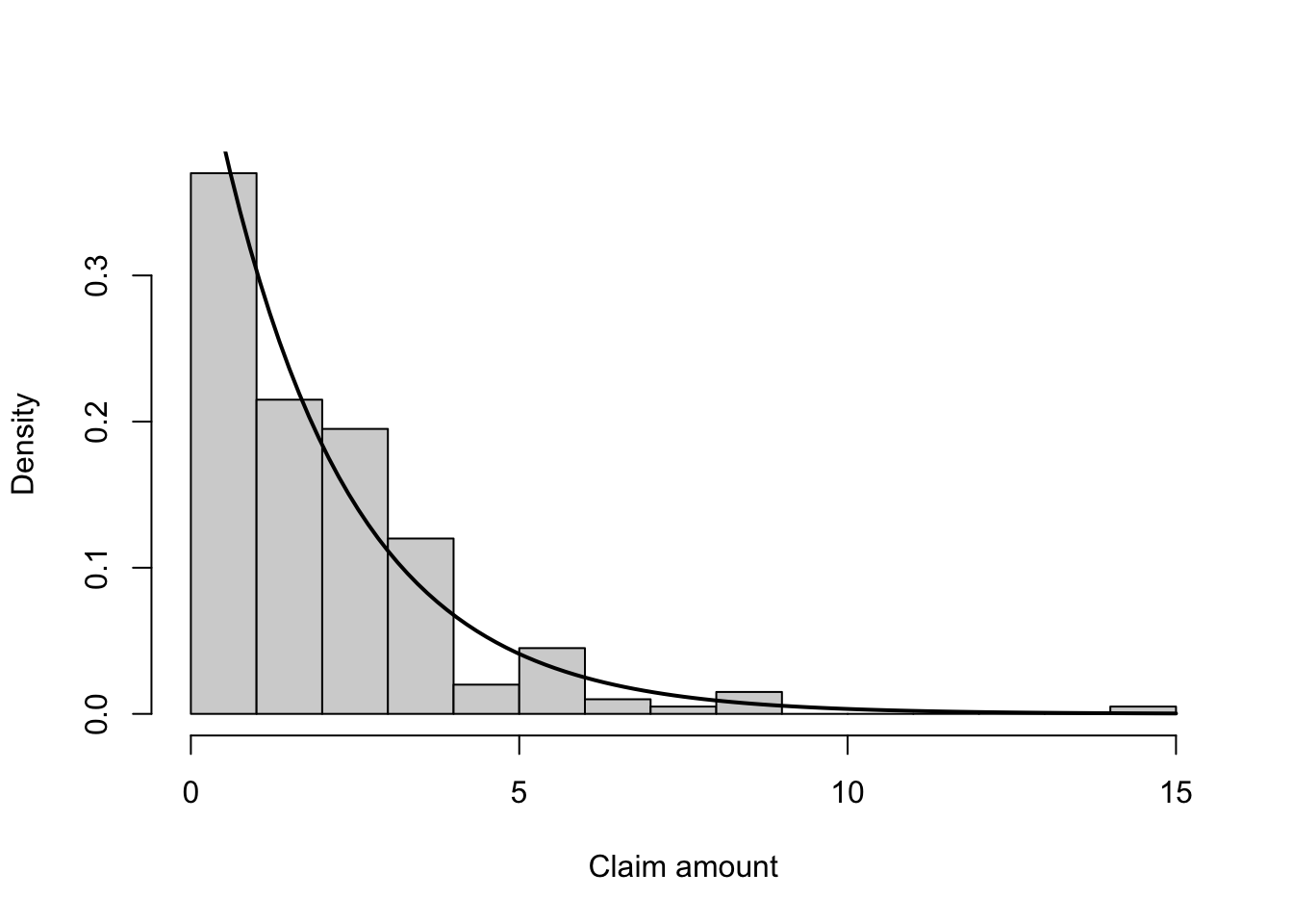
Figure 1.3: Histogram of a simulated sample from an Exponential distribution.

The histogram follows the same general pattern as the theoretical density function. Most observations are concentrated near zero, while progressively fewer observations occur as the claim amount increases. Small irregularities are expected because the histogram is based on a finite random sample rather than the entire population.

As the sample size increases, the histogram more closely resembles the theoretical probability density function. This illustrates one of the fundamental ideas of statistics: empirical distributions converge towards their underlying probability distributions as more observations become available.

Modelling Consideration

A simulated sample never reproduces the theoretical distribution exactly. Random variation is expected, particularly for small samples. The agreement between the histogram and the theoretical density generally improves as the sample size increases.

1.2.6 Memoryless Property and Transition

One of the most distinctive features of the Exponential distribution is its memoryless property.

Suppose that \(X\) represents the time until the next insurance claim is reported. If no claim has occurred during the first \(s\) units of time, the probability that an additional waiting time of at least \(t\) units is required is

\[ \Pr(X>s+t \mid X>s). \]

For the Exponential distribution,

\[ \Pr(X>s+t \mid X>s) = \Pr(X>t), \]

for all \(s,t>0\).

This result shows that the future waiting time does not depend on how long one has already waited. In other words, the process has no memory.

Key Idea

The Exponential distribution is the only continuous probability distribution possessing the memoryless property. This property makes it particularly useful for modelling waiting times between independent random events.

The memoryless property is important in reliability theory, queueing models, and stochastic processes. However, it is generally not an appropriate assumption for modelling insurance claim amounts, because the size of a claim is not naturally interpreted as a waiting time. For this reason, the Exponential distribution is often viewed as an introductory loss model rather than a realistic model for many insurance portfolios.

Transition

The Exponential distribution provides a mathematically simple model for non-negative random variables. However, its single parameter limits the range of shapes that it can represent. Many insurance portfolios exhibit greater variability and stronger right skewness than the Exponential distribution can accommodate.

The next section introduces the Gamma distribution, which extends the Exponential distribution by introducing an additional shape parameter. This extra flexibility enables the Gamma distribution to model a much wider variety of insurance claim data while retaining many desirable mathematical properties.

1.3 Gamma Distribution

1.3.1 Motivation and Definition

In the previous section, we introduced the Exponential distribution as the simplest continuous probability model for non-negative random variables. It is widely used to model waiting times and claim amounts because of its mathematical simplicity and tractable properties. However, the Exponential distribution has only one parameter and therefore has limited flexibility. Once the average claim size is specified, the shape of the distribution is completely determined.

In practice, insurance claim amounts often display a wider variety of shapes than the Exponential distribution can represent. Some portfolios consist mainly of many small claims with only a few moderate claims, while others exhibit a gradual rise to a peak before tapering into a long right tail. A more flexible model is therefore required to accommodate these different patterns.

The Gamma distribution extends the Exponential distribution by introducing an additional parameter that controls the shape of the density. This additional flexibility allows the Gamma distribution to model a much broader range of positively skewed claim-size distributions while retaining many attractive mathematical properties.

The Gamma distribution is one of the most widely used continuous probability models in actuarial science. It is commonly applied to

individual claim amounts with moderate positive skewness;
aggregate waiting times until several events occur;
claim severities in general insurance;
reliability and survival analysis; and
stochastic models involving the sum of several waiting times.

Compared with the Exponential distribution, the Gamma distribution provides a richer family of distributions that can better represent observed insurance data while remaining mathematically tractable.

Key Idea

The Exponential distribution describes the waiting time until one event occurs.

The Gamma distribution generalises this idea by describing the waiting time until several independent events occur. Consequently, it provides a much more flexible model for insurance losses and waiting-time phenomena.

Throughout this section we assume that

\[ X \sim \operatorname{Gamma}(\alpha,\lambda), \]

where

\(\alpha>0\) is the shape parameter, and
\(\lambda>0\) is the rate parameter.

These two parameters together determine both the location and the shape of the distribution.

Definition

Definition 1.4 A continuous random variable \(X\) is said to follow a Gamma distribution with shape parameter \(\alpha>0\) and rate parameter \(\lambda>0\) if its probability density function is

\[ f_X(x)= \frac{\lambda^\alpha} {\Gamma(\alpha)} x^{\alpha-1} e^{-\lambda x}, \qquad x>0. \]

We write

\[ X\sim\operatorname{Gamma}(\alpha,\lambda). \]

The support of the distribution is

\[ x>0. \]

Since claim amounts cannot be negative, the Gamma distribution naturally satisfies one of the fundamental requirements of a loss distribution by assigning zero probability to negative values.

Compared with the Exponential distribution, the Gamma distribution introduces one additional parameter, allowing the density to assume many different shapes. This flexibility makes it particularly useful for modelling insurance claim sizes.

1.3.2 The Gamma Function and Probability Density Function

At first sight, the probability density function of the Gamma distribution appears more complicated than that of the Exponential distribution because it contains the symbol \(\Gamma(\alpha)\). Before studying the distribution itself, it is helpful to understand the meaning of this function.

The Gamma function is a mathematical function that extends the factorial function from positive integers to all positive real numbers. Recall that the factorial of a positive integer is defined by

\[ n!=n(n-1)(n-2)\cdots2\times1. \]

For example,

\[ 3!=6,\qquad 4!=24,\qquad 5!=120. \]

The factorial is only defined for positive integers. The Gamma function extends this idea so that expressions analogous to factorials can be evaluated for any positive real number.

Definition 1.5 The Gamma function is defined by

\[ \Gamma(\alpha) =\int_0^\infty x^{\alpha-1}e^{-x},dx, \qquad \alpha>0. \]

Although this definition involves an improper integral, modern statistical software evaluates the Gamma function efficiently and accurately. In practice, users rarely compute the integral directly.

The Gamma function satisfies an important recursive relationship,

\[ \Gamma(\alpha+1) =\alpha,\Gamma(\alpha). \]

This identity plays a central role in deriving many properties of the Gamma distribution.

For positive integers, repeated application of this identity gives

\[ \Gamma(n) =(n-1)!. \]

For example,

\[ \Gamma(1)=1, \]

\[ \Gamma(2)=1!, \]

\[ \Gamma(3)=2!, \]

and

\[ \Gamma(5)=4!=24. \]

Consequently, the Gamma function is a direct extension of the factorial function.

Interpretation

The Gamma function appears in the denominator of the probability density function because it serves as a normalising constant. Its role is to ensure that the total area under the probability density function equals one,

\[ \int_0^\infty f_X(x),dx=1. \]

Without the Gamma function, the proposed density would not represent a valid probability distribution.

Probability Density Function

Using the Gamma function, the probability density function of a Gamma random variable is

\[ f_X(x) =\frac{\lambda^\alpha} {\Gamma(\alpha)} x^{\alpha-1} e^{-\lambda x}, \qquad x>0. \]

The density consists of four components, each contributing to the overall shape of the distribution.

The term \(\lambda^\alpha\) adjusts the scale of the density according to the rate parameter.
The term \(x^{\alpha-1}\) governs the behaviour near the origin and largely determines the overall shape.
The exponential term \(e^{-\lambda x}\) causes the density to decrease as \(x\) becomes large.
The Gamma function \(\Gamma(\alpha)\) ensures that the density integrates to one.

Unlike the Exponential distribution, whose shape is fixed, the Gamma distribution can take many different forms depending on the values of \(\alpha\) and \(\lambda\). As a result, it is capable of representing a much wider range of insurance claim distributions.

Modelling Consideration

The Gamma distribution is often regarded as the first practical extension of the Exponential distribution. By introducing a second parameter, it provides substantially greater flexibility while remaining mathematically tractable, making it one of the most frequently used continuous distributions in actuarial science.

1.3.3 Properties of the Gamma Distribution

The Gamma distribution possesses several mathematical properties that make it particularly useful in actuarial modelling. These properties allow us to calculate probabilities, summarise the distribution through its moments, and derive many important results used in insurance applications.

Throughout this section, let

\[ X \sim \operatorname{Gamma}(\alpha,\lambda), \]

where \(\alpha>0\) is the shape parameter and \(\lambda>0\) is the rate parameter.

Probability Calculations

Unlike the Exponential distribution, the cumulative distribution function (cdf) of the Gamma distribution does not generally have a simple closed-form expression. Instead, probabilities are obtained from the Gamma cumulative distribution function, which is implemented in most statistical software.

The distribution function is

\[ F_X(x)=P(X\le x) =\int_0^x \frac{\lambda^\alpha}{\Gamma(\alpha)} t^{\alpha-1}e^{-\lambda t}\,dt, \qquad x>0. \]

Consequently,

\[ P(X\le x)=F_X(x), \]

\[ P(X>x)=1-F_X(x), \]

and for any \(0<a<b\),

\[ P(a<X\le b) = F_X(b)-F_X(a). \]

In practice, these probabilities are evaluated numerically using statistical software. For example, in R the cumulative distribution function is computed using the command

pgamma(x, shape = alpha, rate = lambda)

which returns the probability \(P(X\le x)\).

Interpretation

The cumulative distribution function represents the probability that the claim amount does not exceed a specified value. Consequently, it can be used to estimate the proportion of claims expected to fall below a policy limit or deductible.

Quantiles

The quantile function is the inverse of the cumulative distribution function. For a probability level \(0<p<1\), the \(100p\)th percentile, denoted by \(x_p\), satisfies

\[ P(X\le x_p)=p. \]

Equivalently,

\[ x_p=F^{-1}(p). \]

Since the Gamma distribution has no simple inverse cumulative distribution function, quantiles are obtained numerically.

For example,

the median is obtained by setting \(p=0.5\);
the 95th percentile is obtained by setting \(p=0.95\); and
the 99th percentile is obtained by setting \(p=0.99\).

These quantities are particularly important in insurance because they are closely related to risk measures such as Value-at-Risk (VaR).

In R, Gamma quantiles are obtained using

qgamma(p, shape = alpha, rate = lambda)

Moments

Moments describe important characteristics of a probability distribution, including its centre, variability and shape.

The \(r\)th raw moment (moment about the origin) of a Gamma random variable is

\[ E(X^r) = \frac{\Gamma(\alpha+r)} {\lambda^r\Gamma(\alpha)}, \qquad r>0. \]

From this expression, several important summary measures follow immediately.

The mean is

\[ E(X) = \frac{\alpha}{\lambda}, \]

which represents the expected claim amount.

The variance is

\[ \operatorname{Var}(X) = \frac{\alpha}{\lambda^2}, \]

while the standard deviation is

\[ SD(X) = \frac{\sqrt{\alpha}}{\lambda}. \]

The coefficient of variation is therefore

\[ CV = \frac{SD(X)}{E(X)} = \frac{1}{\sqrt{\alpha}}. \]

An attractive feature of the Gamma distribution is that the coefficient of variation depends only on the shape parameter. As \(\alpha\) increases, the relative variability decreases, producing a more concentrated distribution around its mean.

The coefficient of skewness is

\[ \gamma_1 = \frac{2}{\sqrt{\alpha}}. \]

Consequently, larger values of \(\alpha\) produce distributions that are less skewed, whereas smaller values of \(\alpha\) correspond to strongly right-skewed claim distributions.

Interpretation

The shape parameter \(\alpha\) controls much more than the appearance of the density curve. It also determines the relative variability and skewness of the distribution. As \(\alpha\) increases, the distribution becomes less variable relative to its mean and gradually approaches a more symmetric shape.

Moment Generating Function

The moment generating function (mgf) provides an alternative way of describing a probability distribution. It is particularly useful for deriving moments and studying sums of independent random variables.

The moment generating function of a Gamma random variable is

\[ M_X(t) = E(e^{tX}) = \left( 1-\frac{t}{\lambda} \right)^{-\alpha}, \qquad t<\lambda. \]

The mgf has the same general form as that of the Exponential distribution, differing only in the exponent \(-\alpha\).

This simple expression is one reason why the Gamma distribution is widely used in actuarial science. It allows many theoretical results to be derived with relative ease, including the distribution of sums of independent Gamma random variables, which will be discussed later in this chapter.

Summary of Important Properties

Table Table 1.3 summarises the principal mathematical properties of the Gamma distribution.

Table 1.3: Principal mathematical properties of the Gamma distribution.

Property	Result
Support	\(x>0\)
Mean	\(\displaystyle \frac{\alpha}{\lambda}\)
Variance	\(\displaystyle \frac{\alpha}{\lambda^2}\)
Standard deviation	\(\displaystyle \frac{\sqrt{\alpha}}{\lambda}\)
Coefficient of variation	\(\displaystyle \frac{1}{\sqrt{\alpha}}\)
Coefficient of skewness	\(\displaystyle \frac{2}{\sqrt{\alpha}}\)
\(r\)th raw moment	\(\displaystyle \frac{\Gamma(\alpha+r)}{\lambda^r\Gamma(\alpha)}\)
Moment generating function	\(\displaystyle \left(1-\frac{t}{\lambda}\right)^{-\alpha},\quad t<\lambda\)

1.3.4 Visualisation and Simulation of the Gamma Distribution

Visualisation provides valuable insight into how the Gamma distribution behaves and how its parameters influence the shape of the density. Although the probability density function defines the distribution mathematically, graphs often provide a more intuitive understanding of the relationship between the parameters and the resulting claim-size distribution.

Recall that the probability density function is

\[ f(x)=\frac{\lambda^\alpha}{\Gamma(\alpha)} x^{\alpha-1}e^{-\lambda x}, \qquad x>0. \]

Unlike the Exponential distribution, whose shape is completely determined once the rate parameter is specified, the Gamma distribution has two parameters. Consequently, the density can exhibit a much wider range of shapes.

Effect of the Shape Parameter

The shape parameter \(\alpha\) primarily determines the overall shape of the distribution.

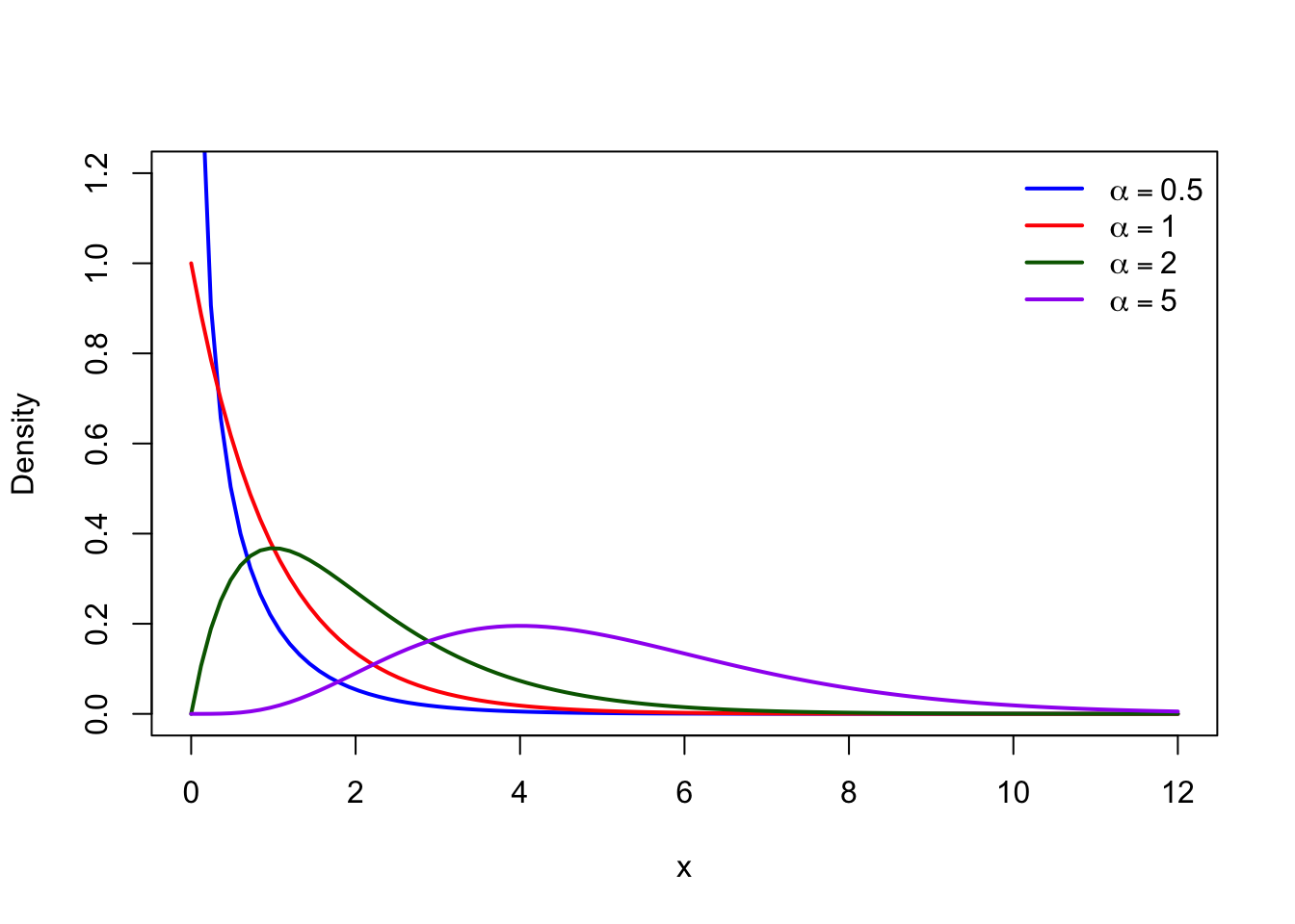
When \(\alpha<1\), the density is highest near the origin and decreases rapidly, indicating that very small claim amounts occur most frequently.
When \(\alpha=1\), the Gamma distribution reduces to the Exponential distribution.
When \(\alpha>1\), the density initially increases to a peak before gradually decreasing, producing a unimodal distribution that often provides a more realistic model for insurance claim amounts.

As the shape parameter increases, the distribution becomes less skewed and more concentrated around its mean.

Figure Figure 1.4 illustrates the effect of varying the shape parameter while keeping the rate parameter fixed.

Code

curve(dgamma(x, shape = 0.5, rate = 1),
      from = 0, to = 12,
      ylim = c(0,1.2),
      lwd = 2,
      col = "blue",
      xlab = "x",
      ylab = "Density")

curve(dgamma(x, shape = 1, rate = 1),
      add = TRUE,
      lwd = 2,
      col = "red")

curve(dgamma(x, shape = 2, rate = 1),
      add = TRUE,
      lwd = 2,
      col = "darkgreen")

curve(dgamma(x, shape = 5, rate = 1),
      add = TRUE,
      lwd = 2,
      col = "purple")

legend("topright",
       legend = c(expression(alpha==0.5),
                  expression(alpha==1),
                  expression(alpha==2),
                  expression(alpha==5)),
       col = c("blue","red","darkgreen","purple"),
       lwd = 2,
       bty = "n")

Figure 1.4: Gamma density functions for various values of the shape parameter.

Interpretation

The shape parameter controls the form of the distribution.

As \(\alpha\) increases, the density shifts away from zero, the peak becomes more pronounced, and the distribution becomes less positively skewed. This flexibility allows the Gamma distribution to model a wide variety of claim-size distributions using the same probability model.

Effect of the Rate Parameter

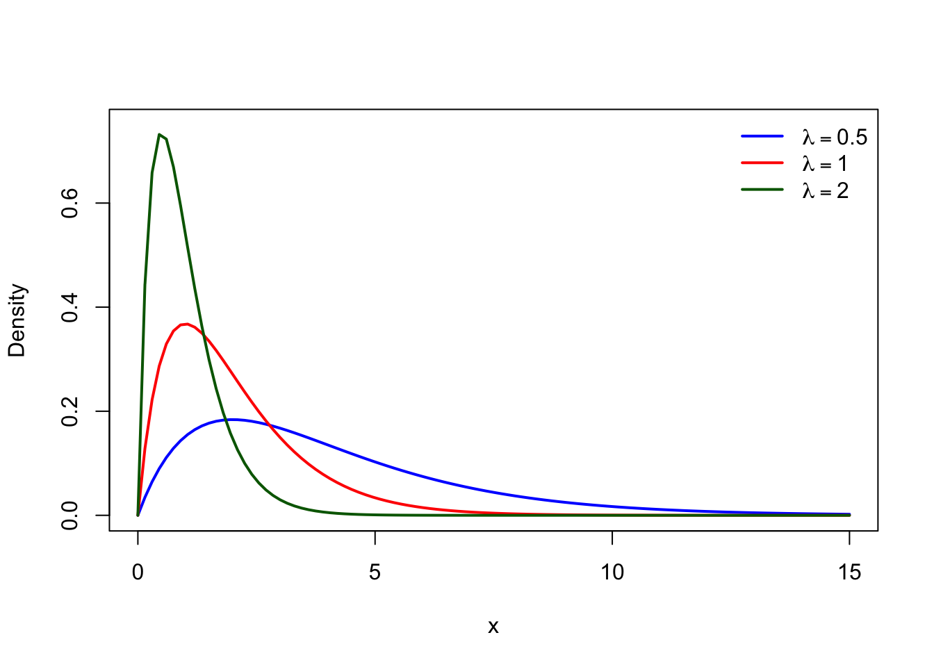
The rate parameter \(\lambda\) controls the scale of the distribution.

For a fixed value of \(\alpha\),

increasing \(\lambda\) concentrates the distribution closer to zero;
decreasing \(\lambda\) spreads the distribution over a wider range of values.

Since

\[ E(X)=\frac{\alpha}{\lambda}, \]

larger values of \(\lambda\) correspond to smaller expected claim amounts.

Figure Figure 1.5 illustrates the effect of changing the rate parameter while holding the shape parameter constant.

Code

curve(dgamma(x, shape = 2, rate = 0.5),
      from = 0, to = 15,
      ylim = c(0,0.75),
      lwd = 2,
      col = "blue",
      xlab = "x",
      ylab = "Density")

curve(dgamma(x, shape = 2, rate = 1),
      add = TRUE,
      lwd = 2,
      col = "red")

curve(dgamma(x, shape = 2, rate = 2),
      add = TRUE,
      lwd = 2,
      col = "darkgreen")

legend("topright",
       legend = c(expression(lambda==0.5),
                  expression(lambda==1),
                  expression(lambda==2)),
       col = c("blue","red","darkgreen"),
       lwd = 2,
       bty = "n")

Figure 1.5: Gamma density functions for various values of the rate parameter.

Interpretation

The rate parameter determines how quickly the density decreases.

A larger rate parameter produces smaller expected claim amounts, whereas a smaller rate parameter allows the distribution to extend further into the right tail.

Simulating Gamma Random Variables in R

Simulation provides a practical way to understand the behaviour of probability distributions. By generating a large random sample, we can compare the simulated data with the theoretical density and observe how random variation influences the sample.

In R, random observations from a Gamma distribution are generated using the rgamma() function.

rgamma(n, shape = alpha, rate = lambda)

where

n is the sample size;
shape specifies \(\alpha\); and
rate specifies \(\lambda\).

Example

The following code generates 1,000 observations from a Gamma distribution with shape parameter \(\alpha=2\) and rate parameter \(\lambda=0.5\).

Code

set.seed(2026)

claims <- rgamma(1000,
                 shape = 2,
                 rate = 0.5)

head(claims)

[1] 4.4106841 0.9381746 0.1209163 1.5892773 4.3531267 6.0539799

Code

summary(claims)

    Min.  1st Qu.   Median     Mean  3rd Qu.     Max. 
 0.09488  1.95118  3.36569  4.06124  5.46403 20.74259

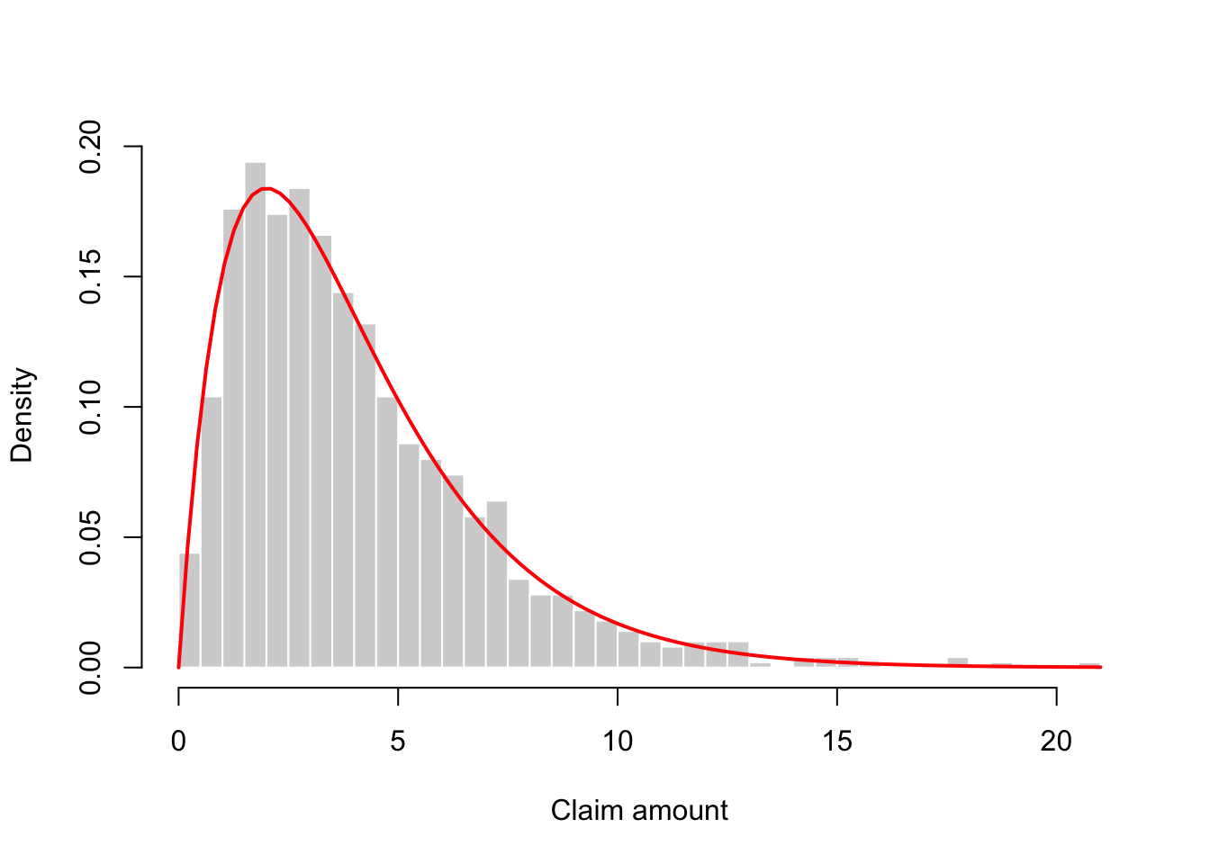
A histogram of the simulated observations can then be compared with the theoretical density.

Code

hist(claims,
     probability = TRUE,
     breaks = 30,
     col = "lightgray",
     border = "white",
     xlab = "Claim amount",
     main = "")

curve(dgamma(x,
             shape = 2,
             rate = 0.5),
      add = TRUE,
      col = "red",
      lwd = 2)

Figure 1.6: Simulated Gamma observations with theoretical density.

The histogram closely follows the theoretical density, although small differences remain because the observations represent only one random sample. If the sample size is increased, the histogram becomes progressively closer to the theoretical curve, illustrating the Law of Large Numbers.

Modelling Consideration

Simulation enables actuaries to investigate the behaviour of loss models when analytical calculations become difficult or impossible. In later chapters, simulated Gamma claim amounts will be combined with frequency models to study aggregate losses and insurance risk.

1.3.5 Summary

The Gamma distribution is one of the most important continuous probability models in actuarial science. It extends the Exponential distribution by introducing a shape parameter, allowing a much wider range of positively skewed distributions to be represented. Its tractable mathematical properties, flexible shape, and ease of simulation make it particularly suitable for modelling many types of insurance claim amounts.

Although the Gamma distribution provides substantially greater flexibility than the Exponential distribution, it is still not appropriate for every insurance application. In particular, some portfolios exhibit claim-size distributions with much heavier right tails than the Gamma distribution can adequately capture.

Looking Ahead

In the next two sections, we introduce two additional continuous loss distributions that address different modelling needs.

The Lognormal distribution is particularly useful when claim amounts arise from multiplicative effects and exhibit substantial positive skewness. It has become one of the most widely used models for individual claim severities because it often provides an excellent fit to real insurance data.

The Pareto distribution, in contrast, is specifically designed to model extremely large losses. Its heavy right tail makes it especially suitable for catastrophic claims, liability insurance, and reinsurance applications, where rare but exceptionally large losses play a dominant role in risk management.

Together, the Gamma, Lognormal, and Pareto distributions form a powerful collection of continuous models that enable actuaries to represent a broad spectrum of insurance loss distributions, from routine claims to extreme catastrophic events.

1.4 Lognormal Distribution

1.4.1 Motivation and Definition

The Gamma distribution provides a flexible model for many insurance claim amounts and is capable of representing a wide range of positively skewed data. Nevertheless, some classes of insurance business exhibit an even greater degree of variability than the Gamma distribution can adequately capture. In particular, certain claim portfolios contain a large number of relatively small claims together with a small proportion of exceptionally large losses. These distributions are characterised by a long right tail that extends much further than that of the Gamma distribution.

Examples include bodily injury claims, medical expenses, liability claims, and property losses resulting from natural catastrophes. In these situations, the claim amount is often influenced by the combined effect of many independent factors, such as the severity of an accident, medical costs, inflation, legal expenses, and the duration of settlement. Since these factors tend to interact multiplicatively rather than additively, the resulting claim amounts are frequently well described by the Lognormal distribution.

The Lognormal distribution has become one of the most widely used continuous probability models in actuarial science. Its ability to model highly skewed claim-size distributions makes it particularly suitable for many insurance applications, including

individual claim severities;
medical and healthcare costs;
liability and bodily injury claims;
property insurance losses; and
financial losses involving multiplicative growth.

Unlike the Gamma distribution, whose shape is controlled by two parameters acting directly on the density, the Lognormal distribution is defined through a transformation of the Normal distribution. Specifically, a random variable follows a Lognormal distribution if its natural logarithm follows a Normal distribution.

This relationship provides both mathematical convenience and practical flexibility, making the Lognormal distribution one of the most important severity models in actuarial practice.

Key Idea

A random variable is Lognormally distributed if its logarithm is Normally distributed.

In other words,

\[ X \text{ is Lognormal } \quad\Longleftrightarrow\quad \ln(X) \text{ is Normal.} \]

This simple transformation produces a distribution that is always positive and naturally exhibits the strong right skewness commonly observed in insurance claim amounts.

Throughout this section we assume that

\[ X\sim LN(\mu,\sigma^2), \]

where

\(\mu\) is the mean of the logarithm of the random variable; and
\(\sigma>0\) is the standard deviation of the logarithm.

It is important to note that these parameters describe the distribution of \(\ln(X)\) rather than the distribution of \(X\) itself.

Definition

Before defining the Lognormal distribution formally, recall that many natural and financial phenomena are better explained by multiplicative rather than additive processes.

For example, the total cost of an insurance claim may depend on several factors, including

repair costs,
labour charges,
inflation,
exchange rates,
legal expenses, and
medical treatment costs.

These factors combine by multiplying their effects rather than simply adding fixed amounts. When many independent multiplicative effects act together, the resulting distribution is often approximately Lognormal.

Definition 1.6 A continuous random variable \(X\) is said to follow a Lognormal distribution with parameters \(\mu\) and \(\sigma>0\) if

\[ \ln(X)\sim N(\mu,\sigma^2). \]

Equivalently,

\[ X=e^Y, \qquad Y\sim N(\mu,\sigma^2). \]

We write

\[ X\sim LN(\mu,\sigma^2). \]

The support of the distribution is

\[ x>0. \]

Since

\[ e^Y>0 \]

for every real value of \(Y\), the Lognormal distribution assigns zero probability to negative values. This makes it a natural candidate for modelling claim severities, survival times, and other non-negative random variables.

1.4.2 Relationship with the Normal Distribution

The Lognormal distribution is derived directly from the Normal distribution through an exponential transformation.

Suppose that

\[ Y\sim N(\mu,\sigma^2). \]

If we define

\[ X=e^Y, \]

then

\[ X\sim LN(\mu,\sigma^2). \]

Conversely,

\[ Y=\ln(X) \]

follows a Normal distribution.

This relationship is illustrated schematically as

\[ \boxed{ Y \sim N(\mu,\sigma^2) } \qquad \xrightarrow{\;X=e^Y\;} \qquad \boxed{ X \sim LN(\mu,\sigma^2) } \]

The exponential transformation converts the symmetric Normal distribution into a positively skewed distribution whose values are strictly positive.

Interpretation

The parameters \(\mu\) and \(\sigma\) describe the distribution of the logarithm of the claim amount, not the claim amount itself.

Consequently,

\(\mu\) is not the mean claim size.
\(\sigma\) is not the standard deviation of claim amounts.

Instead, they describe the location and variability of \(\ln(X)\).

1.4.3 Probability Model and Parameter Interpretation

Probability Density Function

\[ X\sim LN(\mu,\sigma^2), \]

then its probability density function is

\[ f(x) = \frac{1} {x\sigma\sqrt{2\pi}} \exp\left[ -\frac{(\ln x-\mu)^2} {2\sigma^2} \right], \qquad x>0. \]

Although this expression appears more complicated than the densities of the Exponential or Gamma distributions, each component has a clear interpretation.

The denominator \(x\) arises from the logarithmic transformation.
The parameter \(\mu\) determines the location of the distribution.
The parameter \(\sigma\) controls the spread and degree of skewness.
The exponential term ensures that the density decreases as observations move away from the centre of the distribution on the logarithmic scale.

Because of the logarithmic transformation, the density is always positively skewed. Unlike the Gamma distribution, whose skewness decreases steadily as the shape parameter increases, the Lognormal distribution can maintain substantial skewness even when the variability is moderate.

Interpretation of the Parameters

The Lognormal distribution contains two parameters, each serving a different purpose.

The Location Parameter \(\mu\)

The parameter \(\mu\) determines the location of the distribution on the logarithmic scale.

Increasing \(\mu\)

shifts the distribution towards larger claim amounts;
increases the mean claim size; and
leaves the overall shape largely unchanged.

Conversely, decreasing \(\mu\) shifts the entire distribution towards smaller values.

The Scale Parameter \(\sigma\)

The parameter \(\sigma\) measures the variability of the logarithm of the claim amount.

As \(\sigma\) increases,

the distribution becomes more dispersed;
the right tail becomes substantially longer;
extremely large claims become more likely; and
the distribution becomes increasingly positively skewed.

Small values of \(\sigma\) produce densities that are relatively concentrated, whereas large values produce distributions with considerable variability and a pronounced heavy right tail.

Modelling Consideration

The parameter \(\sigma\) has a profound influence on the tail behaviour of the Lognormal distribution. Even moderate increases in \(\sigma\) can substantially increase the probability of observing exceptionally large insurance claims. This characteristic makes the Lognormal distribution particularly useful for modelling claim severities in liability, health, and property insurance.

Cumulative Distribution Function

Unlike the Exponential distribution, the cumulative distribution function of the Lognormal distribution cannot be expressed in elementary closed form. Instead, probabilities are obtained through the cumulative distribution function of the Normal distribution.

\[ X\sim LN(\mu,\sigma^2), \]

then

\[ P(X\le x) = P(\ln X\le \ln x) = \Phi\left( \frac{\ln x-\mu}{\sigma} \right), \qquad x>0, \]

where \(\Phi(\cdot)\) denotes the cumulative distribution function of the standard Normal distribution.

Consequently,

\[ F(x) = \Phi\left( \frac{\ln x-\mu}{\sigma} \right), \qquad x>0. \]

Since the cumulative distribution function is expressed in terms of the standard Normal distribution, all probability calculations can be performed using standard statistical tables or statistical software.

For example, in R the cumulative distribution function is evaluated using

plnorm(x, meanlog = mu, sdlog = sigma)

which returns the probability

\[ P(X\le x). \]

This close connection with the Normal distribution greatly simplifies probability calculations and is one of the principal reasons for the widespread use of the Lognormal distribution in actuarial modelling.

Properties of the Lognormal Distribution

The Lognormal distribution possesses several mathematical properties that make it particularly suitable for modelling insurance claim severities. In contrast to the Gamma distribution, the Lognormal distribution has no moment generating function because of its heavy right tail. Nevertheless, its moments have simple closed-form expressions and play an important role in actuarial applications.

Throughout this section, let

\[ X\sim LN(\mu,\sigma^2), \]

where \(\mu\) and \(\sigma\) are the parameters of the logarithm of the random variable.

Probability Calculations

Since

\[ \ln(X)\sim N(\mu,\sigma^2), \]

probability calculations for the Lognormal distribution can be transformed into equivalent calculations involving the Normal distribution.

The cumulative distribution function is

\[ F(x) = P(X\le x) = \Phi\left( \frac{\ln x-\mu}{\sigma} \right), \qquad x>0, \]

where \(\Phi(\cdot)\) denotes the cumulative distribution function of the standard Normal distribution.

Consequently,

\[ P(X\le x) = F(x), \]

\[ P(X>x) = 1-F(x), \]

and

\[ P(a<X\le b) = F(b)-F(a). \]

In R, these probabilities are computed using

plnorm(x, meanlog = mu, sdlog = sigma)

which returns the probability

\[ P(X\le x). \]

Interpretation

Because probabilities are evaluated through the Normal distribution, many calculations for the Lognormal distribution reduce to standard Normal probability calculations after taking logarithms.

Quantiles

The \(100p\)th percentile of a Lognormal distribution is defined by

\[ P(X\le x_p)=p. \]

Since

\[ F(x) = \Phi\left( \frac{\ln x-\mu}{\sigma} \right), \]

the quantile function is

\[ x_p = \exp\left[ \mu+\sigma\Phi^{-1}(p) \right]. \]

Thus,

the median is

\[ \exp(\mu), \]

the 95th percentile is

\[ \exp\left[\mu+1.645\sigma\right], \]

and the 99th percentile is

\[ \exp\left[\mu+2.326\sigma\right]. \]

Unlike the mean, the median depends only on the location parameter \(\mu\).

In R, Lognormal quantiles are obtained using

qlnorm(p, meanlog = mu, sdlog = sigma)

The quantile function is particularly important in insurance because high percentiles are frequently used to determine capital requirements and risk measures such as Value-at-Risk (VaR).

1.4.4 Properties, Visualisation, and Simulation

Moments

One attractive feature of the Lognormal distribution is that all positive moments exist and have simple closed-form expressions.

The \(r\)th raw moment is

\[ E(X^r) = \exp\left( r\mu+\frac{r^2\sigma^2}{2} \right), \qquad r>0. \]

Several important summary measures follow immediately.

The mean is

\[ E(X) = \exp\left( \mu+\frac{\sigma^2}{2} \right), \]

which is always greater than the median.

The variance is

\[ \operatorname{Var}(X) = \exp\left( 2\mu+\sigma^2 \right) \left( e^{\sigma^2}-1 \right). \]

The standard deviation is therefore

\[ SD(X) = \sqrt{\operatorname{Var}(X)}. \]

The coefficient of variation is

\[ CV = \sqrt{e^{\sigma^2}-1}, \]

which depends only on the scale parameter \(\sigma\).

The coefficient of skewness is

\[ \gamma_1 = \left( e^{\sigma^2}+2 \right) \sqrt{e^{\sigma^2}-1}. \]

Unlike the Gamma distribution, the skewness of the Lognormal distribution increases rapidly as \(\sigma\) increases. Consequently, even moderate values of \(\sigma\) can produce distributions with extremely long right tails.

Interpretation

The parameter \(\sigma\) controls not only the spread of the distribution but also its tail behaviour. Larger values of \(\sigma\) produce greater variability, stronger positive skewness, and a higher probability of extremely large insurance claims.

Moment Generating Function

The Lognormal distribution differs fundamentally from the Exponential and Gamma distributions in that its moment generating function does not exist for any positive value of \(t\).

That is,

\[ M_X(t) = E(e^{tX}) \]

does not converge for any

\[ t>0. \]

This result arises because the exponential function grows more rapidly than the Lognormal density decreases in the right tail.

Although the moment generating function does not exist, all ordinary moments exist and can be obtained directly from the expression for the \(r\)th raw moment.

Important

The absence of a moment generating function does not imply that the Lognormal distribution lacks finite moments. In fact, moments of every order exist. Only the moment generating function fails to converge because of the heavy right tail of the distribution.

Summary of Important Properties

Table Table 1.4 summarises the principal mathematical properties of the Lognormal distribution.

Table 1.4: Important properties of the Lognormal distribution.

Property	Result
Support	\(x>0\)
Median	\(\exp(\mu)\)
Mean	\(\displaystyle \exp\left(\mu+\frac{\sigma^2}{2}\right)\)
Variance	\(\displaystyle \exp(2\mu+\sigma^2)\left(e^{\sigma^2}-1\right)\)
Standard deviation	\(\displaystyle \sqrt{\exp(2\mu+\sigma^2)\left(e^{\sigma^2}-1\right)}\)
Coefficient of variation	\(\displaystyle \sqrt{e^{\sigma^2}-1}\)
Coefficient of skewness	\(\displaystyle (e^{\sigma^2}+2)\sqrt{e^{\sigma^2}-1}\)
\(r\)th raw moment	\(\displaystyle \exp\left(r\mu+\frac{r^2\sigma^2}{2}\right)\)
Moment generating function	Does not exist for \(t>0\)

The Lognormal distribution combines mathematical tractability with the ability to model highly skewed claim-size distributions. These characteristics explain why it has become one of the most widely used severity distributions in actuarial science. In the next section, we visualise the Lognormal distribution, investigate the effects of its parameters, and demonstrate how random samples can be generated using R.

Visualising the Lognormal Distribution

Visualisation provides an intuitive understanding of how the Lognormal distribution behaves and how its parameters influence the shape of the claim-size distribution. In insurance applications, claim amounts are typically positive and right-skewed, with many small claims and a small number of very large claims. The Lognormal distribution is particularly useful in this setting because it can represent this type of heavy right tail.

Recall that a random variable \(X\) follows a Lognormal distribution if

\[ Y=\log(X) \]

follows a Normal distribution:

\[ Y \sim N(\mu,\sigma^2). \]

The probability density function of \(X\) is

\[ f(x)= \frac{1}{x\sigma\sqrt{2\pi}} \exp \left\{ -\frac{(\log x-\mu)^2}{2\sigma^2} \right\}, \qquad x>0. \]

The Lognormal distribution has two parameters:

\(\mu\), which controls the location of the distribution on the logarithmic scale.
\(\sigma\), which controls the spread and the degree of skewness.

Unlike the Gamma distribution, the Lognormal distribution is always positively skewed. However, changing \(\sigma\) can substantially alter the heaviness of the right tail.

Effect of the Location Parameter

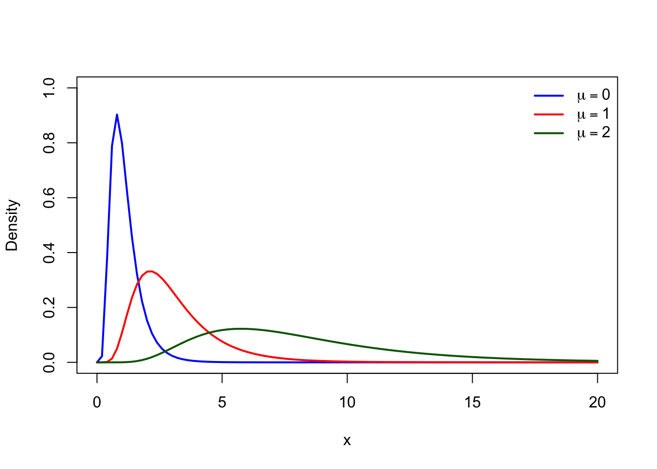
The parameter \(\mu\) determines the location of the distribution. Increasing \(\mu\) shifts the distribution to the right while preserving its general shape.

A larger value of \(\mu\) implies larger typical claim amounts because the median of the distribution is

\[ \operatorname{Median}(X)=e^\mu. \]

Figure Figure 1.7 illustrates the effect of changing \(\mu\) while keeping \(\sigma\) fixed.

Code

curve(dlnorm(x, meanlog = 0, sdlog = 0.5),
      from = 0, to = 20,
      ylim = c(0,1),
      lwd = 2,
      col = "blue",
      xlab = "x",
      ylab = "Density")

curve(dlnorm(x, meanlog = 1, sdlog = 0.5),
      add = TRUE,
      lwd = 2,
      col = "red")

curve(dlnorm(x, meanlog = 2, sdlog = 0.5),
      add = TRUE,
      lwd = 2,
      col = "darkgreen")

legend("topright",
       legend = c(expression(mu==0),
                  expression(mu==1),
                  expression(mu==2)),
       col = c("blue","red","darkgreen"),
       lwd = 2,
       bty = "n")

Figure 1.7: Lognormal density functions for various values of the location parameter.

Effect of the Scale Parameter

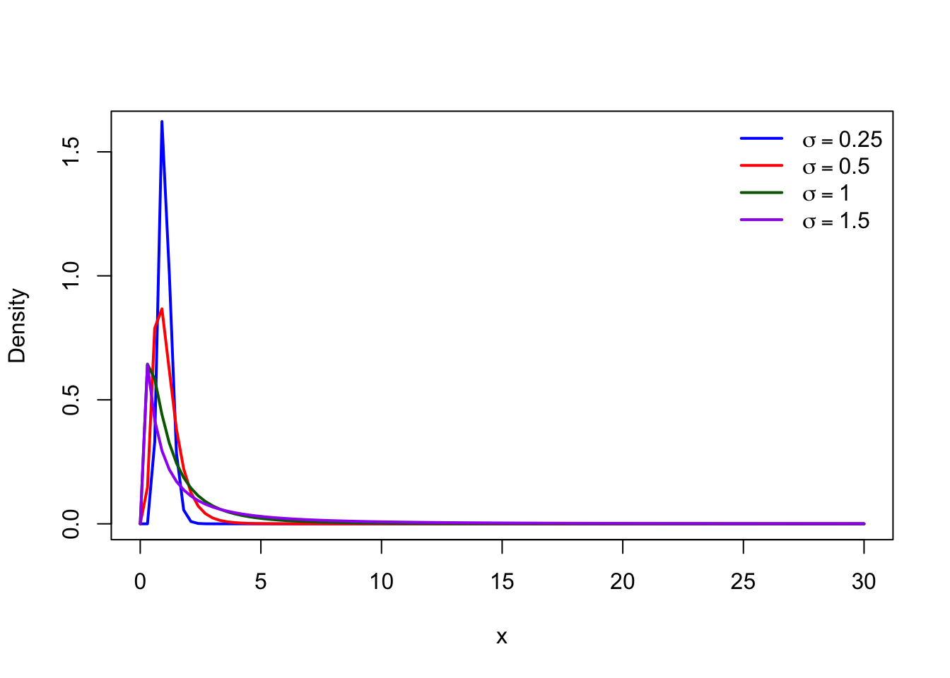
The parameter \(\sigma\) determines the variability on the logarithmic scale and has a strong influence on skewness.

A small value of \(\sigma\) produces a distribution concentrated around its typical value.
A larger value of \(\sigma\) produces greater dispersion and a heavier right tail.
In insurance applications, a larger \(\sigma\) represents greater uncertainty and a higher probability of extreme claim amounts.

Figure Figure 1.8 illustrates the effect of changing \(\sigma\) while keeping \(\mu\) fixed.

Code

curve(dlnorm(x, meanlog = 0, sdlog = 0.25),
      from = 0, to = 30,
      ylim = c(0,1.6),
      lwd = 2,
      col = "blue",
      xlab = "x",
      ylab = "Density")

curve(dlnorm(x, meanlog = 0, sdlog = 0.5),
      add = TRUE,
      lwd = 2,
      col = "red")

curve(dlnorm(x, meanlog = 0, sdlog = 1),
      add = TRUE,
      lwd = 2,
      col = "darkgreen")

curve(dlnorm(x, meanlog = 0, sdlog = 1.5),
      add = TRUE,
      lwd = 2,
      col = "purple")

legend("topright",
       legend = c(expression(sigma==0.25),
                  expression(sigma==0.5),
                  expression(sigma==1),
                  expression(sigma==1.5)),
       col = c("blue","red","darkgreen","purple"),
       lwd = 2,
       bty = "n")

Figure 1.8: Lognormal density functions for various values of the scale parameter.

Interpretation

The parameter \(\sigma\) plays an important role in insurance loss modelling because it controls the probability of observing very large claims.

As \(\sigma\) increases, the distribution becomes more dispersed and the right tail becomes heavier. Therefore, two Lognormal distributions with the same median may produce substantially different risk measures, such as Value-at-Risk (\(\operatorname{VaR}\)) and Tail Value-at-Risk (\(\operatorname{TVaR}\)).

Simulating Random Variables from the Lognormal Distribution

Simulation is an important technique in actuarial risk modelling because it allows us to generate artificial claim amounts and study the behaviour of a portfolio.

Since the Lognormal distribution is obtained by exponentiating a Normal random variable, simulation follows a simple two-step procedure:

Generate observations from a Normal distribution:

\[ Y_i \sim N(\mu,\sigma^2). \]

Transform the simulated values:

\[ X_i=e^{Y_i}. \]

The resulting values follow a Lognormal distribution:

\[ X_i\sim\operatorname{Lognormal}(\mu,\sigma^2). \]

The following code simulates \(1,000\) claim amounts from a Lognormal distribution with \(\mu=2\) and \(\sigma=1\).

Code

set.seed(123)

n <- 1000

claims <- rlnorm(n,
                 meanlog = 2,
                 sdlog = 1)

hist(claims,
     breaks = 40,
     probability = TRUE,
     xlab = "Claim amount",
     main = "")

curve(dlnorm(x,
             meanlog = 2,
             sdlog = 1),
      add = TRUE,
      lwd = 2)

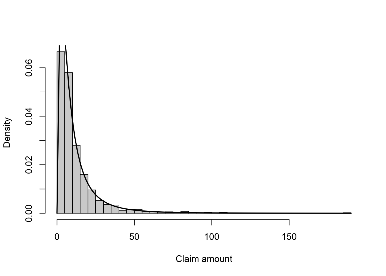
Figure 1.9: Simulated claim amounts from a Lognormal distribution.

The histogram demonstrates the typical behaviour of insurance claim data:

Most simulated claims are relatively small.
A small number of observations produce extremely large claim amounts.
The distribution has a long right tail, which is a key feature of many insurance loss distributions.

1.4.5 Transition to Heavy-Tailed Loss Distributions

Both the Gamma and Lognormal distributions are widely used for modelling insurance claim severity. The Gamma distribution provides flexibility through its shape parameter, while the Lognormal distribution naturally captures multiplicative variation and heavier right tails.

However, some insurance portfolios contain extreme losses that are even larger than those predicted by these distributions. Examples include:

catastrophic property losses,
large liability claims,
natural disaster events.

For such situations, models with heavier tails are required.

The Pareto distribution is one of the most important heavy-tailed distributions in actuarial science. Unlike the Gamma and Lognormal distributions, which have exponentially decreasing tails, the Pareto distribution has a polynomially decreasing tail:

\[ P(X>x)\sim x^{-\alpha}, \qquad x\rightarrow\infty. \]

This slower decay means that extremely large losses occur with higher probability.

The progression of severity models can therefore be viewed as:

\[ \text{Gamma} \longrightarrow \text{Lognormal} \longrightarrow \text{Pareto}. \]

The Gamma distribution provides a flexible model for moderately skewed losses, the Lognormal distribution captures greater skewness and variability, and the Pareto distribution is designed for situations where extreme losses dominate the risk profile.

1.5 Pareto Distribution

1.5.1 Motivation and Definition

Insurance claim amounts are often highly right-skewed. Most claims are relatively small, but a small number of claims can be exceptionally large. These large claims are particularly important in insurance because they can have a substantial effect on the total amount paid by an insurer.

The exponential and Gamma distributions can provide useful models for claim amounts, but they may not adequately represent situations in which very large claims occur more frequently than these distributions would suggest. This motivates the use of distributions with heavier tails.

The Pareto distribution is one of the most widely used heavy-tailed distributions for modelling insurance losses. It is particularly useful for large claims, liability losses, catastrophic losses, and reinsurance applications.

A random variable \(X\) has a Pareto distribution with parameters \(\alpha > 0\) and \(\lambda > 0\), denoted by

\[ X \sim \operatorname{Pa}(\alpha,\lambda), \]

if its probability density function is

\[ f_X(x) =\frac{\alpha\lambda^\alpha} {(\lambda+x)^{\alpha+1}}, \qquad x>0. \]

The parameter \(\alpha\) controls the heaviness of the tail, while \(\lambda\) determines the scale of the distribution. The distinction between these two parameters is important when interpreting the behaviour of Pareto losses.

The corresponding cumulative distribution function is

\[ F_X(x) =1- \left( \frac{\lambda}{\lambda+x} \right)^\alpha, \qquad x>0. \]

Consequently, the survival function is

\[ \overline{F}_X(x) =\Pr(X>x)= \left( \frac{\lambda}{\lambda+x} \right)^\alpha. \]

The survival function is particularly useful in insurance because it directly describes the probability that a claim exceeds a specified amount.

1.5.2 Probability Model and Parameter Interpretation

For \(X \sim \operatorname{Pa}(\alpha,\lambda)\), the probability that a claim falls between two positive amounts \(a\) and \(b\), where \(0<a<b\), is

\[ \Pr(a<X\leq b) =F_X(b)-F_X(a). \]

Using the survival function,

\[ \Pr(a<X\leq b) =\left( \frac{\lambda}{\lambda+a} \right)^\alpha -\left( \frac{\lambda}{\lambda+b} \right)^\alpha. \]

Similarly, the probability that a claim exceeds \(x\) is

\[ \Pr(X>x) =\left( \frac{\lambda}{\lambda+x} \right)^\alpha. \]

This exceedance probability is central to the modelling of large insurance claims.

The shape parameter \(\alpha\) determines how quickly the tail probability decreases. A smaller value of \(\alpha\) produces a heavier tail and therefore gives relatively greater probability to very large claims. A larger value of \(\alpha\) produces a lighter tail.

The scale parameter \(\lambda\) controls the overall scale of the claim amounts. Increasing \(\lambda\) shifts the distribution towards larger claim amounts while retaining the same basic tail shape determined by \(\alpha\).

The quantile function can be obtained by solving

\[ F_X(x)=p. \]

This gives

\[ Q_X(p) =\lambda \left[ (1-p)^{-1/\alpha}-1 \right], \qquad 0<p<1. \]

In particular, the median is

\[ \operatorname{Med}(X) =\lambda \left( 2^{1/\alpha}-1 \right). \]

The quantile function is useful for describing high claim amounts and for calculating risk measures based on specified probability levels.

1.5.3 Properties and Heavy-Tail Behaviour

The properties of the Pareto distribution depend strongly on the value of the shape parameter \(\alpha\).

The mean and variance of \(X\) are

\[ \mathrm{E}[X] =\frac{\lambda}{\alpha-1}, \qquad \alpha>1, \]

and

\[ \operatorname{Var}(X) =\frac{\alpha\lambda^2} {(\alpha-1)^2(\alpha-2)}, \qquad \alpha>2. \]

Thus, the mean does not exist when \(\alpha\leq1\), and the variance does not exist when \(\alpha\leq2\). This illustrates an important feature of heavy-tailed distributions: sufficiently high moments may fail to exist.

More generally, the \(r\)-th moment about the origin is

\[ \mathrm{E}[X^r] = \frac{\Gamma(\alpha-r)\Gamma(1+r)} {\Gamma(\alpha)} \lambda^r, \qquad 0<r<\alpha. \]

Therefore, the \(r\)-th moment exists only when

\[ r<\alpha. \]

The moment generating function of \(X\) is not finite for any positive value of \(t\). Consequently, the Pareto distribution does not have a moment generating function in the usual positive neighbourhood of zero.

When \(\alpha>3\), the coefficient of skewness is

\[ \frac{2(\alpha+1)}{\alpha-3} \sqrt{\frac{\alpha-2}{\alpha}}. \]

The dependence of the moments on \(\alpha\) provides a useful interpretation of the shape parameter. As \(\alpha\) decreases, the tail becomes heavier and the distribution becomes increasingly influenced by extreme observations.

The survival function also makes the heavy-tail behaviour clear. For large \(x\),

\[ \overline{F}_X(x) =\left( \frac{\lambda}{\lambda+x} \right)^\alpha \sim \lambda^\alpha x^{-\alpha}. \]

Thus, the tail decreases approximately according to a power law rather than exponentially. This slow decay is the defining feature that makes the Pareto distribution useful for modelling unusually large insurance losses.

An important conditional tail property is also useful for reinsurance calculations. Let \(X\sim\operatorname{Pa}(\alpha,\lambda)\). Then

\[ X-w\mid X>w \sim \operatorname{Pa}(\alpha,\lambda+w). \]

This property shows that, conditional on a claim exceeding a threshold \(w\), the excess claim \(X-w\) remains within the Pareto family. This makes the distribution particularly convenient for modelling claims above deductibles, attachment points, or other insurance thresholds.

1.5.4 Visualisation, Simulation, and Actuarial Applications

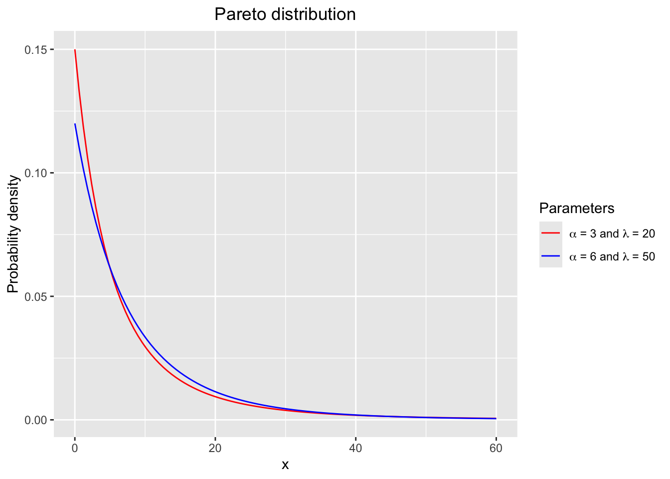
Visualisation provides a useful way to examine how the Pareto distribution behaves as its parameters change. In particular, the shape parameter \(\alpha\) has a strong effect on the tail of the distribution.

For example, the following figure compares two Pareto distributions with different parameter values.

Code

library(actuar)
library(ggplot2)

ggplot(data.frame(x = c(0, 60)), aes(x = x)) +
  labs(y = "Probability density", x = "x") +
  ggtitle("Pareto distribution") +
  theme(plot.title = element_text(hjust = 0.5)) +
  stat_function(
    fun = dpareto,
    args = list(shape = 3, scale = 20),
    aes(colour = "alpha = 3, lambda = 20")
  ) +
  stat_function(
    fun = dpareto,
    args = list(shape = 6, scale = 50),
    aes(colour = "alpha = 6, lambda = 50")
  ) +
  scale_colour_manual(
    "Parameters",
    values = c("red", "blue"),
    labels = c(
      expression(paste(alpha, " = 3 and ", lambda, " = 20")),
      expression(paste(alpha, " = 6 and ", lambda, " = 50"))
    )
  )

Probability density functions of Pareto distributions with different shape and scale parameters.

The Pareto distribution can also be simulated in R. Simulation makes it possible to examine the occurrence of extreme observations and to compare simulated claim amounts with the theoretical distribution.

The Pareto distribution is particularly useful when modelling claim amounts for which very large observations are important. Applications include:

large individual claims;
liability losses;
catastrophic losses; and
reinsurance claims above a specified attachment point.

For example, the conditional tail property

\[ X-w\mid X>w \sim \operatorname{Pa}(\alpha,\lambda+w) \]

provides a convenient representation for excess losses in reinsurance.

The Pareto distribution can therefore be used not only to model individual claim amounts but also to describe the behaviour of claims in the upper tail of the loss distribution.

1.5.5 Comparison and Transition to Aggregate Losses

In practice, the lognormal and Pareto distributions can provide better fits to claim amounts than the exponential and Gamma distributions, particularly when the data contain a substantial number of large claims.

The Pareto distribution has an especially simple and interpretable tail structure. However, its heavy-tail behaviour may also make it inappropriate when the observed claim data do not exhibit sufficiently heavy tails. Model selection should therefore be based on the characteristics of the data rather than on the theoretical advantages of a particular distribution.

A comparison of the fitted exponential, Gamma, lognormal, and Pareto distributions can help assess which model provides the most appropriate representation of observed claim amounts.

Other loss distributions that are useful in practice include the Burr, Weibull, and loggamma distributions.

Once a suitable distribution has been selected for an individual claim amount \(X\), the next step is to consider the total loss arising from a portfolio of claims. If \(N\) denotes the number of claims and \(X_1,X_2,\ldots,X_N\) denote the corresponding claim amounts, the aggregate loss can be represented by

\[ S=\sum_{i=1}^{N}X_i. \]

This moves the analysis from individual loss distributions to aggregate loss modelling, which is the basis for studying the total claims incurred by an insurance portfolio.

1.6 Worked Example: Fitting Loss Distributions to Claim Amounts

The following example illustrates how different loss distributions can be fitted to observed insurance claim amounts. In particular, it provides an opportunity to compare the Pareto distribution with the exponential, Gamma, and lognormal distributions. The example also highlights the importance of the upper tail when modelling insurance losses.

Example 1.2 (Fitting Loss Distributions to Claim Amounts) Consider a data set consisting of 200 claim amounts in one year from a general insurance portfolio.

Calculate the sample mean and sample standard deviation.
Use the method of moments to fit these data with exponential, Gamma, lognormal, and Pareto distributions.
Calculate the boundaries for groups or bins so that the expected number of claims in each bin is 20 under the fitted exponential distribution.
Count the observed claim amounts in each bin.
Using these bin boundaries, find the expected number of claims when the data are fitted with the Gamma, lognormal, and Pareto distributions.
Plot a histogram of the data together with the fitted distributions.
Comment on the goodness of fit of the fitted distributions.

Solution

Suppose that

\[ \sum_{i=1}^n x_i=206046.4 \]

and

\[ \sum_{i=1}^n x_i^2=1,472,400,135, \]

where \(n=200\).

The sample mean is

\[ \bar{x} = \frac{\sum_{i=1}^n x_i}{n} = \frac{206046.4}{200} = 1030.232. \]

The sample variance is

\[ s^2 =\frac{1}{n-1} \left[ \sum_{i=1}^n x_i^2 -\frac{\left(\sum_{i=1}^n x_i\right)^2}{n} \right] =6332284. \]

Therefore, the sample standard deviation is

\[ s=2516.403. \]

The standard deviation is substantially larger than the sample mean. This provides an initial indication of strong right-skewness and suggests that unusually large claims may have an important influence on the data.

1.6.1 Fitting the Distributions

We use the method of moments by matching the theoretical mean and variance of each distribution to the corresponding sample moments.

For an exponential distribution \(X\sim\operatorname{Exp}(\lambda)\)),

\[ \mathrm{E}[X]=\frac{1}{\lambda}. \]

Thus, the method-of-moments estimate is

\[ \tilde{\lambda} = \frac{1}{\bar{x}} = 0.000971. \]

For a Gamma distribution \(X\sim\mathcal{G}(\alpha,\lambda)\), using the rate parameterisation,

\[ \mathrm{E}[X]=\frac{\alpha}{\lambda}, \qquad \operatorname{Var}(X)=\frac{\alpha}{\lambda^2}. \]

The method-of-moments estimates are therefore

\[ \begin{aligned} \tilde{\alpha} &= \left(\frac{\bar{x}}{s}\right)^2 =0.167614,\\ \tilde{\lambda} &= \frac{\tilde{\alpha}}{\bar{x}} =0.000163. \end{aligned} \]

For a lognormal distribution \(X\sim\operatorname{LN}(\mu,\sigma^2)\),

\[ \mathrm{E}[X] =e^{\mu+\sigma^2/2}, \]

and

\[ \operatorname{Var}(X) =\left(e^{\sigma^2}-1\right)e^{2\mu+\sigma^2}. \]

The resulting method-of-moments estimates are

\[ \begin{aligned} \tilde{\sigma} &= \sqrt{ \ln\left( \frac{s^2}{\bar{x}^2}+1 \right) } = 1.393218, \\ \tilde{\mu} &= \ln(\bar{x}) - \frac{\tilde{\sigma}^2}{2} = 5.967012. \end{aligned} \]

For the Pareto distribution \(X\sim\operatorname{Pa}(\alpha,\lambda)\)),

\[ \mathrm{E}[X] =\frac{\lambda}{\alpha-1}, \qquad \alpha>1, \]

and

\[ \operatorname{Var}(X) =\frac{\alpha\lambda^2} {(\alpha-1)^2(\alpha-2)}, \qquad \alpha>2. \]

Matching these moments to the sample mean and variance gives

\[ \begin{aligned} \tilde{\alpha} &= 2 \left( \frac{s^2}{\bar{x}^2} \right) \frac{1} {\left(\frac{s^2}{\bar{x}^2}-1\right)} = 2.402731, \\ \tilde{\lambda} &= \bar{x}(\tilde{\alpha}-1) = 1445.138. \end{aligned} \]

The fitted Pareto distribution therefore has a shape parameter of approximately \(2.40\). Since this value is only slightly greater than \(2\), the model has a relatively heavy tail, while its variance remains finite.

Constructing the Claim-Size Groups

To compare the fitted distributions with the observed data, divide the 200 claims into 10 groups, with an expected 20 claims in each group under the fitted exponential distribution.

The upper boundary \(\operatorname{upbd}_j\) of group \(j\) satisfies

\[ \Pr(X\leq \operatorname{upbd}_j) =\frac{j}{10}, \qquad j=1,2,\ldots,9. \]

For the fitted exponential distribution,

\[ \Pr(X\leq x) =1-e^{-\tilde{\lambda}x}. \]

Hence,

\[ \operatorname{upbd}_j =-\frac{1}{\tilde{\lambda}} \ln\left(1-\frac{j}{10}\right). \]

These boundaries divide the observed claims into intervals containing the observed frequencies shown below.

Range	Observation	Exponential	Gamma	Lognormal	Pareto
\((0,109]\)	60	20	109.4	36.0	31.9
\((109,230]\)	31	20	14.3	34.4	27.8
\((230,367]\)	25	20	9.7	26.0	24.2
\((367,526]\)	17	20	7.8	20.5	21.2
\((526,714]\)	14	20	6.8	16.6	18.6
\((714,944]\)	13	20	6.3	13.9	16.4
\((944,1240]\)	6	20	6.2	11.9	14.6
\((1240,1658]\)	7	20	6.5	10.8	13.2
\((1658,2372]\)	10	20	7.7	10.4	12.5
\((2372,\infty)\)	17	20	25.4	19.5	19.4

The expected number of claims in an interval \((a,b]\) under a fitted distribution is

\[ 200\Pr(a<X\leq b). \]

For the fitted Pareto distribution, this becomes

\[ 200 \left[ \left( \frac{\tilde{\lambda}}{\tilde{\lambda}+a} \right)^{\tilde{\alpha}} - \left( \frac{\tilde{\lambda}}{\tilde{\lambda}+b} \right)^{\tilde{\alpha}} \right]. \]

The same procedure can be applied to the other fitted distributions.

Interpretation

The observed data show a substantial concentration of relatively small claims, together with a number of very large claims. In particular, 17 claims are greater than \(2,372\), and five claims, representing \(2.5\%\) of the observations, are greater than \(10,000\).

This behaviour is difficult to capture with the exponential distribution. The exponential model assigns the same expected frequency to each of the ten groups and therefore does not reflect the concentration of observations among small claims and the presence of unusually large claims.

The Gamma distribution also provides a poor fit. It substantially overestimates the number of very small claims and underestimates several groups in the middle and upper portions of the distribution.

The lognormal and Pareto distributions provide a substantially better representation of the observed claim amounts. In particular, their heavier tails allow them to assign greater probability to large claims.

The comparison illustrates an important point in loss modelling: a distribution should not be selected solely because it provides a reasonable fit to the central part of the data. Its ability to represent the upper tail is also important, because a relatively small number of very large claims can have a substantial impact on an insurer’s total losses.

This example therefore provides a practical motivation for using heavy-tailed distributions such as the lognormal and Pareto distributions in insurance loss modelling.

1.6.2 R Code: Fitting the Loss Distributions

The claim amounts are stored in the vector claims. The data are then converted to a data frame for use with ggplot2.

Code

claims <- c(
  31.08942156, 915.0259362, 32.02379562, 885.875451, 9314.100797,
  707.1738866, 2114.362486, 601.5827866, 435.3788135, 49.80179619,
  1802.38382, 211.636439, 153.5984719, 60.05966992, 48.17157697,
  948.7234626, 132.4273109, 151.710815, 2967.961036, 735.4149332,
  304.5807587, 50.53311069, 224.7665546, 356.1809438, 475.7668441,
  3044.149513, 13.50664894, 67.98274449, 304.1439966, 238.000105,
  399.0798263, 149.28078, 128.2848379, 21.42027718, 73.31426732,
  49.46882791, 667.5327275, 44.67360185, 14894.07839, 660.7614307,
  100.7628628, 632.2812391, 42.90884777, 66.17693135, 50.69454132,
  186.8781667, 168.5408615, 151.739978, 2419.532354, 434.4564032,
  69.03460232, 162.6698593, 226.6110395, 33.61503495, 233.027996,
  3244.945893, 354.2534813, 78.61052744, 231.566614, 283.0206491,
  457.6785426, 134.2933058, 61.34265063, 38.25691912, 1578.909048,
  441.6199826, 761.4177777, 275.6978588, 521.0355916, 2189.62783,
  117.2667885, 240.3403153, 672.4512938, 753.8958019, 84.98883079,
  3665.417976, 60.35977515, 4.01933309, 14.95951366, 196.7146403,
  153.7133165, 98.31875053, 104.4486324, 358.9205878, 2.254986331,
  2059.603959, 37.63898608, 56.48944035, 1143.082948, 410.7585516,
  12.65402986, 19.83322514, 1305.134797, 2019.360735, 1286.98479,
  8892.182131, 5.814518749, 296.1551295, 86.75308161, 486.7851405,
  7.491389798, 180.3255281, 1414.297748, 524.4628208, 1042.690334,
  1291.481474, 115.4950998, 360.6310737, 3233.716838, 149.5191039,
  8.845837473, 83.87296324, 42.99614517, 623.9704853, 45.74990074,
  144.2449793, 368.575642, 866.9272545, 57.61592921, 1812.231315,
  2229.998754, 3448.332888, 11313.34721, 1492.498856, 196.7262571,
  71.11817601, 425.0614483, 38.28653048, 44.5090016, 308.8781657,
  19080.51749, 82.0761393, 250.083523, 79.07492042, 183.8697686,
  33.83160391, 22.78218299, 698.9541648, 32.75427003, 457.0104919,
  112.1715567, 396.7155234, 195.0240781, 1863.185385, 181.6441121,
  59.08733655, 96.39004191, 824.730184, 155.8215162, 11.85510661,
  870.8679502, 425.3133045, 854.7296474, 254.3108892, 664.3320107,
  56.26120752, 378.244016, 2069.431495, 3121.0901, 844.4337594,
  746.3853675, 1851.469633, 431.7060232, 333.325481, 22.23970102,
  662.3816888, 117.7590057, 570.4412829, 1127.035306, 246.2686183,
  1467.568867, 34.89187112, 237.5761693, 349.4503967, 229.3362849,
  934.6926561, 162.9254408, 58.28497172, 12803.04726, 15.94904189,
  959.9543402, 5853.878979, 537.3974253, 75.30572883, 718.6597521,
  633.8214438, 363.0338076, 95.8476266, 80.3178653, 286.7121763,
  6367.453408, 321.567711, 21.51838022, 599.4712958, 246.7007073,
  13863.78181, 214.7342597, 234.3212952, 958.916179, 165.2521385
)

dat <- data.frame(claims = claims)

n <- length(claims)
xbar <- mean(claims)
s <- sd(claims)

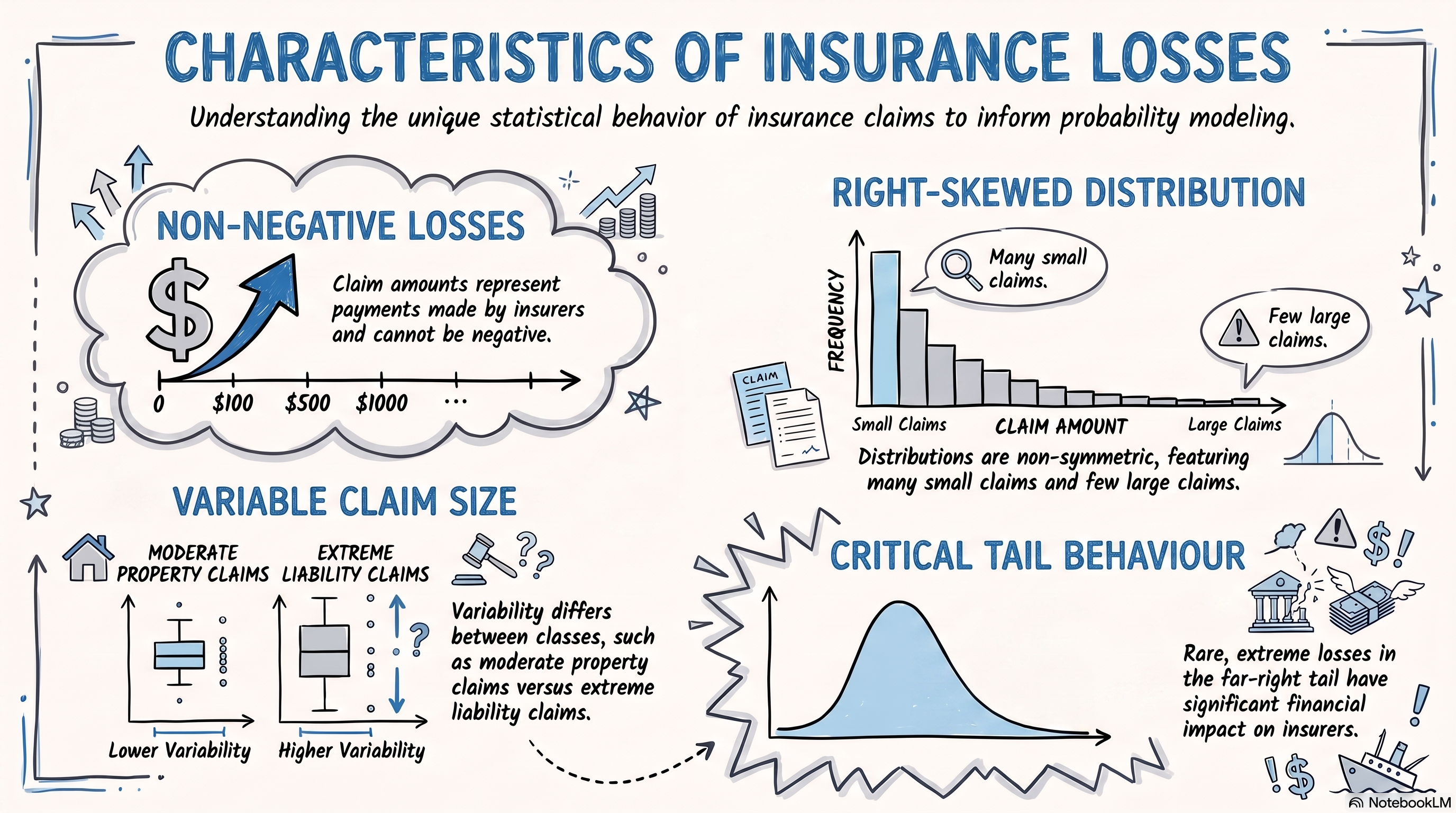
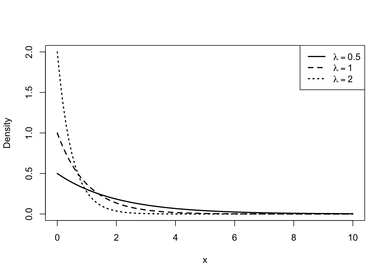
The sample mean and standard deviation can be obtained directly:

Code

c(
  n = n,
  mean = xbar,
  sd = s
)

       n     mean       sd 
 200.000 1030.232 2516.403

Method-of-Moments Estimates

We now estimate the parameters of the four candidate distributions.

For the exponential distribution,

\[ \hat{\lambda}_{\mathrm{Exp}} =\frac{1}{\bar{x}}. \]

For the Gamma distribution,

\[ \hat{\alpha}_{\mathrm{Gamma}} =\left(\frac{\bar{x}}{s}\right)^2, \qquad \hat{\lambda}_{\mathrm{Gamma}} =\frac{\hat{\alpha}_{\mathrm{Gamma}}}{\bar{x}}. \]

For the lognormal distribution,

\[ \hat{\sigma}_{\mathrm{LN}} =\sqrt{ \ln\left( 1+\frac{s^2}{\bar{x}^2} \right) }, \]

and

\[ \hat{\mu}_{\mathrm{LN}} =\ln(\bar{x}) = \frac{\hat{\sigma}_{\mathrm{LN}}^2}{2}. \]

For the Pareto distribution,

\[ \hat{\alpha}_{\mathrm{Pa}} =\frac{2s^2} {s^2-\bar{x}^2}, \]

and

\[ \hat{\lambda}_{\mathrm{Pa}} =\bar{x}(\hat{\alpha}_{\mathrm{Pa}}-1). \]

These estimates can be calculated in R as follows.

Code

# Exponential
lambda_exp <- 1 / xbar

# Gamma
alpha_gamma <- (xbar / s)^2
lambda_gamma <- alpha_gamma / xbar

# Lognormal
sigma_lnorm <- sqrt(log(1 + s^2 / xbar^2))
mu_lnorm <- log(xbar) - sigma_lnorm^2 / 2

# Pareto
alpha_pareto <- 2 * s^2 / (s^2 - xbar^2)
lambda_pareto <- xbar * (alpha_pareto - 1)

estimates <- data.frame(
  Distribution = c(
    "Exponential",
    "Gamma",
    "Lognormal",
    "Pareto"
  ),
  Parameter_1 = c(
    lambda_exp,
    alpha_gamma,
    mu_lnorm,
    alpha_pareto
  ),
  Parameter_2 = c(
    NA,
    lambda_gamma,
    sigma_lnorm,
    lambda_pareto
  )
)

estimates

  Distribution  Parameter_1  Parameter_2
1  Exponential 0.0009706552           NA
2        Gamma 0.1676137495 1.626952e-04
3    Lognormal 5.9670116665 1.393218e+00
4       Pareto 2.4027307020 1.445138e+03

Comparing the Fitted Densities

The fitted distributions can now be compared with the observed claim amounts.

Because the claim distribution is highly right-skewed, the horizontal axis can extend over a wide range. The histogram is therefore shown together with the fitted densities.

Code

library(ggplot2)
library(actuar)

ggplot(dat, aes(x = claims)) +
  geom_histogram(
    aes(y = after_stat(density)),
    bins = 90,
    fill = "grey",
    colour = "black"
  ) +
  stat_function(
    fun = dexp,
    args = list(rate = lambda_exp),
    aes(colour = "Exponential"),
    linewidth = 1
  ) +
  stat_function(
    fun = dgamma,
    args = list(
      shape = alpha_gamma,
      rate = lambda_gamma
    ),
    aes(colour = "Gamma"),
    linewidth = 1
  ) +
  stat_function(
    fun = dlnorm,
    args = list(
      meanlog = mu_lnorm,
      sdlog = sigma_lnorm
    ),
    aes(colour = "Lognormal"),
    linewidth = 1
  ) +
  stat_function(
    fun = dpareto,
    args = list(
      shape = alpha_pareto,
      scale = lambda_pareto
    ),
    aes(colour = "Pareto"),
    linewidth = 1
  ) +
  coord_cartesian(
    xlim = c(0, 5000),
    ylim = c(0, 0.0015)
  ) +
  labs(
    x = "Claim amount",
    y = "Density",
    colour = "Fitted Distributions"
  ) +
  theme_minimal()

Note on the Horizontal Axis

The data contain a small number of exceptionally large claims, with the largest claim being approximately \(19{,}081\), while most claims are substantially smaller. Plotting the entire range of the data would compress the histogram near zero and make it difficult to distinguish the fitted distributions.

For visual comparison, the figure therefore focuses on the main body of the claim distribution by restricting the horizontal axis to \(0\leq x\leq5{,}000\). This restriction is used only for visualisation; all observations, including the largest claims, are retained in the analysis and in the subsequent goodness-of-fit calculations.

Constructing the Claim-Size Groups

To compare the fitted distributions with the observed data, we divide the claims into ten groups. The boundaries are selected so that the fitted exponential distribution assigns probability \(0.1\) to each group.

The first nine boundaries are therefore the exponential quantiles

\[ q_j =F_{\mathrm{Exp}}^{-1} \left(\frac{j}{10}\right), \qquad j=1,\ldots,9. \]

In R:

Code

# Nine finite boundaries plus the lower boundary zero
breaks <- c(
  0,
  qexp(
    (1:9) / 10,
    rate = lambda_exp
  ),
  Inf
)

breaks

 [1]    0.0000  108.5458  229.8896  367.4579  526.2689  714.1024  943.9920
 [8] 1240.3713 1658.0944 2372.1968       Inf

The observed number of claims in each interval is then

Code

observed <- cut(
  claims,
  breaks = breaks,
  right = TRUE,
  include.lowest = TRUE
)

observed_counts <- as.numeric(table(observed))

observed_counts

 [1] 60 31 25 17 14 13  6  7 10 17

Expected Frequencies

For any fitted distribution with CDF \(F\), the expected number of observations in the interval \((a,b]\) is

\[ n\left[F(b)-F(a)\right]. \]

The following function calculates the expected frequencies for a fitted CDF.

Code

expected_counts <- function(breaks, cdf, n) {
  n * diff(cdf(breaks))
}

For the four fitted distributions:

Code

expected_exp <- expected_counts(
  breaks,
  function(x) pexp(x, rate = lambda_exp),
  n
)

expected_gamma <- expected_counts(
  breaks,
  function(x) pgamma(
    x,
    shape = alpha_gamma,
    rate = lambda_gamma
  ),
  n
)

expected_lognormal <- expected_counts(
  breaks,
  function(x) plnorm(
    x,
    meanlog = mu_lnorm,
    sdlog = sigma_lnorm
  ),
  n
)

expected_pareto <- expected_counts(
  breaks,
  function(x) ppareto(
    x,
    shape = alpha_pareto,
    scale = lambda_pareto
  ),
  n
)

The observed and expected frequencies can then be displayed together:

Code

frequency_table <- data.frame(
  Range = levels(observed),
  Observation = observed_counts,
  Exponential = expected_exp,
  Gamma = expected_gamma,
  Lognormal = expected_lognormal,
  Pareto = expected_pareto
)

frequency_table

                 Range Observation Exponential      Gamma Lognormal   Pareto
1              [0,109]          60          20 109.351209  35.82935 31.94317
2            (109,230]          31          20  14.309717  34.56574 27.78045
3            (230,367]          25          20   9.692622  26.14677 24.23276
4            (367,526]          17          20   7.765947  20.43993 21.20592
5            (526,714]          14          20   6.782391  16.55591 18.62739
6            (714,944]          13          20   6.296048  13.84513 16.44617
7       (944,1.24e+03]           6          20   6.182470  11.95451 14.63953
8  (1.24e+03,1.66e+03]           7          20   6.504665  10.74409 13.24216
9  (1.66e+03,2.37e+03]          10          20   7.743835  10.39504 12.49879
10      (2.37e+03,Inf]          17          20  25.371095  19.52352 19.38366

The table provides a direct comparison between the observed claim frequencies and those expected under each fitted model.

Goodness-of-Fit for the Fitted Models

The histogram provides a visual comparison between the observed claim amounts and the fitted distributions. We can also make a more formal comparison using a chi-square goodness-of-fit test.

The same class intervals are used for all four fitted distributions. Let \(O_j\) denote the observed number of claims in group \(j\), and let \(E_j\) denote the expected number of claims under a fitted distribution. The expected number of claims in the interval \((a_{j-1},a_j]\) is

\[ E_j =n\left[ F(a_j)-F(a_{j-1}) \right], \]

where \(F\) is the CDF of the fitted distribution.

The chi-square goodness-of-fit statistic is

\[ \chi^2 =\sum_{j=1}^{k} \frac{(O_j-E_j)^2}{E_j}, \]

where \(k\) is the number of groups.

We can also perform the corresponding chi-square tests. Since the expected frequencies are calculated from the fitted distributions, the test provides a formal assessment of the discrepancy between the observed and expected frequencies.

The null hypothesis for each model is \[H_0:\text{ the observed claim amounts follow the specified fitted distribution},\] while the alternative hypothesis is \[H_1:\text{ the observed claim amounts do not follow the specified fitted distribution}.\]

For the four fitted distributions:

Code

chisq_exp <- sum(
  (observed_counts - expected_exp)^2 /
    expected_exp
)

chisq_gamma <- sum(
  (observed_counts - expected_gamma)^2 /
    expected_gamma
)

chisq_lognormal <- sum(
  (observed_counts - expected_lognormal)^2 /
    expected_lognormal
)

chisq_pareto <- sum(
  (observed_counts - expected_pareto)^2 /
    expected_pareto
)

The resulting chi-square statistics are:

Code

chisq_statistics <- data.frame(
  Distribution = c(
    "Exponential",
    "Gamma",
    "Lognormal",
    "Pareto"
  ),
  Chi_square = c(
    chisq_exp,
    chisq_gamma,
    chisq_lognormal,
    chisq_pareto
  )
)

chisq_statistics

  Distribution Chi_square
1  Exponential  115.70000
2        Gamma   95.17537
3    Lognormal   22.36071
4       Pareto   36.58035

A smaller value of \(\chi^2\) indicates a smaller discrepancy between the observed and expected frequencies and therefore provides evidence of a better fit.

The chi-square test can be performed in R for each fitted model:

Code

test_exp <- chisq.test(
  x = observed_counts,
  p = expected_exp / sum(expected_exp)
)

test_gamma <- chisq.test(
  x = observed_counts,
  p = expected_gamma / sum(expected_gamma)
)

test_lognormal <- chisq.test(
  x = observed_counts,
  p = expected_lognormal / sum(expected_lognormal)
)

test_pareto <- chisq.test(
  x = observed_counts,
  p = expected_pareto / sum(expected_pareto)
)

The test statistics and \(p\)-values can be summarised as follows:

Code

gof_results <- data.frame(
  Distribution = c(
    "Exponential",
    "Gamma",
    "Lognormal",
    "Pareto"
  ),
  Chi_square = c(
    test_exp$statistic,
    test_gamma$statistic,
    test_lognormal$statistic,
    test_pareto$statistic
  ),
  p_value = c(
    test_exp$p.value,
    test_gamma$p.value,
    test_lognormal$p.value,
    test_pareto$p.value
  )
)

gof_results

  Distribution Chi_square      p_value
1  Exponential  115.70000 1.011790e-20
2        Gamma   95.17537 1.482345e-16
3    Lognormal   22.36071 7.803440e-03
4       Pareto   36.58035 3.126480e-05

Comparing the Four Models

The chi-square statistics provide a direct comparison of the discrepancies between the observed and expected frequencies. A smaller chi-square statistic indicates closer agreement between the fitted model and the observed data. Among the four models, the Lognormal distribution gives the smallest value,

\[ \chi^2 = 22.36, \]

followed by the Pareto distribution with \(\chi^2 = 36.58\). The Gamma and Exponential distributions give substantially larger values of \(95.18\) and \(115.70\), respectively. Thus, based on the chi-square statistic, the Lognormal distribution provides the best fit among the four fitted models.

The \(p\)-value provides a formal goodness-of-fit test. At significance level \(\alpha_0\), we reject the fitted model when

\[ p\text{-value}<\alpha_0. \]

For \(\alpha_0=0.05\), the results are

Distribution	\(\chi^2\)	\(p\)-value	Decision
Exponential	115.70	\(1.01\times10^{-20}\)	Reject
Gamma	95.18	\(1.48\times10^{-16}\)	Reject
Lognormal	22.36	\(0.0078\)	Reject
Pareto	36.58	\(3.13\times10^{-5}\)	Reject

Although the Lognormal distribution has the best fit among the four models, its \(p\)-value is still below \(0.05\). Therefore, the chi-square test rejects all four fitted distributions at the 5% significance level. The results suggest that none of the four models provides an adequate fit to the data according to the chi-square goodness-of-fit test.

The numerical results should nevertheless be considered together with the histogram and the frequency table. In particular, the upper tail is important for insurance loss data because a relatively small number of very large claims can have a substantial impact on total losses. The comparison therefore indicates that the Lognormal distribution is the most plausible of the four models considered, but its lack of fit remains statistically significant.