Simple Random Walk Definition

Introduction to Simple Random Walk

A simple random walk \( X_n \) is a fundamental concept in probability theory and stochastic processes. It describes a path where each step taken depends randomly on whether the previous step was positive or negative. Starting from an initial value \( a \), the process moves step by step, with each step increasing or decreasing by 1 with probabilities \( p \) and \( 1 - p \) respectively.

The evolution of \( X_n \) is governed by the accumulation of these random increments or decrements, making it a versatile model for various real-world phenomena such as financial markets, biological systems, and more.

A simple random walk \( X_n \) is a discrete-time stochastic process defined by the following rules:

• \( X_0 = a \), where \( a \) is a constant initial value.

• For \( n \geq 1 \),

  \[ X_n = a + \sum_{i=1}^{n} Z_i, \]

  where \( Z_i \) are independent random variables defined as:

  \[\begin{split} Z_i = \begin{cases} 1, & \text{with probability } p \\ -1, & \text{with probability } q = 1 - p \end{cases} \end{split}\]

In this definition:

• \( p \) is the probability of moving to the next step positively.

• \( q = 1 - p \) is the probability of moving to the next step negatively.

The values \( Z_i \) represent the increments or decrements taken at each step \( n \), contributing to the path \( X_n \) of the random walk.

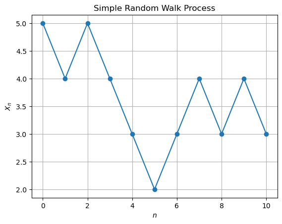
We will simulate this process by flipping a coin to determine the values of \(Z_i\) and then record the output for \(Z_i\) and \(X_n\) in a table form for \(n = 0\) to \(10\) with \(a = 5\).

import random

# Parameters
a = 5
n_steps = 10
p = 0.5  # Probability of Z_i being 1
q = 1 - p  # Probability of Z_i being -1

# Initialize the process
X = [a]
Z = []

# Simulate the random walk
for n in range(1, n_steps + 1):
    Z_i = 1 if random.random() < p else -1
    Z.append(Z_i)
    X.append(X[-1] + Z_i)

# Output the results
print(f"{'n':>2} {'Z_i':>4} {'X_n':>4}")
print(f"{'0':>2} {'-':>4} {X[0]:>4}")
for i in range(1, n_steps + 1):
    print(f"{i:>2} {Z[i-1]:>4} {X[i]:>4}")

# Visualize the process
plt.plot(range(n_steps + 1), X, marker='o')
plt.title('Simple Random Walk Process')
plt.xlabel('$n$')
plt.ylabel('$X_n$')
plt.grid(True)
plt.show()

import random
import matplotlib.pyplot as plt


# Parameters
a = 5
n_steps = 10
p = 0.5  # Probability of Z_i being 1
q = 1 - p  # Probability of Z_i being -1

# Initialize the process
X = [a]
Z = []

# Simulate the random walk
for n in range(1, n_steps + 1):
    Z_i = 1 if random.random() < p else -1
    Z.append(Z_i)
    X.append(X[-1] + Z_i)

# Output the results
print(f"{'n':>2} {'Z_i':>4} {'X_n':>4}")
print(f"{'0':>2} {'-':>4} {X[0]:>4}")
for i in range(1, n_steps + 1):
    print(f"{i:>2} {Z[i-1]:>4} {X[i]:>4}")

# Visualize the process
plt.plot(range(n_steps + 1), X, marker='o')
plt.title('Simple Random Walk Process')
plt.xlabel('$n$')
plt.ylabel('$X_n$')
plt.grid(True)
plt.show()

 n  Z_i  X_n
 0    -    5
 1   -1    4
 2    1    5
 3   -1    4
 4   -1    3
 5   -1    2
 6    1    3
 7    1    4
 8   -1    3
 9    1    4
10   -1    3

f"{'n':>1} {'Z_i':>4} {'X_n':>4}"

'n  Z_i  X_n'

Generating a Sample Path of Simple Random Walk in Python

To simulate and visualize a sample path of a simple random walk in Python, you can follow these steps using NumPy:

1. Import Required Libraries:

import numpy as np
import matplotlib.pyplot as plt

2. Set Parameters:

Define the parameters for the random walk:

np.random.seed(42)  # Setting a random seed for reproducibility
n_steps = 100  # Number of steps in the random walk
p = 0.5  # Probability of moving positively
initial_value = 0  # Starting value of the walk

3. Generate Random Steps

Create an array of random steps \(Z_i\) using NumPy’s random module:

steps = np.random.choice([-1, 1], size=n_steps, p=[1 - p, p])

4. Compute the Random Walk Path

Calculate the cumulative sum to get the path $X_n%:

path = np.cumsum(np.insert(steps, 0, initial_value))

5. Plot the Random Walk

Visualize the generated path using Matplotlib:

plt.figure(figsize=(10, 6))
plt.plot(path, marker='o', linestyle='-')
plt.title('Sample Path of Simple Random Walk')
plt.xlabel('Steps')
plt.ylabel('Value')
plt.grid(True)
plt.show()

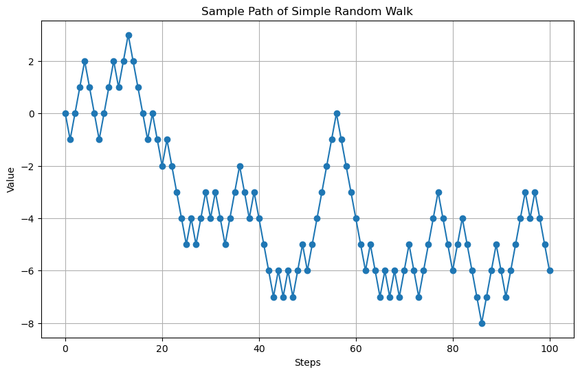
6. Result: Sample Path of Simple Random Walk

Running the above code will generate and display a sample path of a simple random walk:

plt.figure(figsize=(10, 6))
plt.plot(path, marker='o', linestyle='-')
plt.title('Sample Path of Simple Random Walk')
plt.xlabel('Steps')
plt.ylabel('Value')
plt.grid(True)
plt.show()

## Simple Random Walk Simulation in Python

import numpy as np
import matplotlib.pyplot as plt

# Set parameters
np.random.seed(42)  # Setting a random seed for reproducibility
n_steps = 100  # Number of steps in the random walk
p = 0.5  # Probability of moving positively
initial_value = 0  # Starting value of the walk

# Generate random steps
steps = np.random.choice([-1, 1], size=n_steps, p=[1 - p, p])

# Compute the random walk path
path = np.cumsum(np.insert(steps, 0, initial_value))

# Plot the random walk
plt.figure(figsize=(10, 6))
plt.plot(path, marker='o', linestyle='-')
plt.title('Sample Path of Simple Random Walk')
plt.xlabel('Steps')
plt.ylabel('Value')
plt.grid(True)
plt.show()

Generating Multiple Sample Paths of Simple Random Walk in Python

To simulate and visualize multiple sample paths of a simple random walk in Python, you can follow these steps using NumPy:

1. Import Required Libraries:

import numpy as np
import matplotlib.pyplot as plt

2. Set Parameters:

Define the parameters for the random walk:

np.random.seed(42)  # Setting a random seed for reproducibility
n_steps = 100  # Number of steps in each random walk
n_paths = 10  # Number of sample paths
p = 0.5  # Probability of moving positively
initial_value = 0  # Starting value of the walk

3. Generate Random Steps for Multiple Paths

Create an array of random steps \(Z_i\) for multiple paths using NumPy’s random module:

steps = np.random.choice([-1, 1], size=(n_paths, n_steps), p=[1 - p, p])

4. Compute the Random Walk Paths

Calculate the cumulative sum to get the paths \(X_n\) for each sample path:

paths = np.cumsum(np.insert(steps, 0, initial_value, axis=1), axis=1)

5. Plot the Random Walks

Visualize the generated paths using Matplotlib:

plt.figure(figsize=(12, 8))
for i in range(n_paths):
    plt.plot(paths[i], marker='o', linestyle='-', alpha=0.7, label=f'Path {i+1}')
plt.title('Multiple Sample Paths of Simple Random Walk')
plt.xlabel('Steps')
plt.ylabel('Value')
plt.legend()
plt.grid(True)
plt.show()

6. Result: Multiple Sample Paths of Simple Random Walk

Running the above code will generate and display 10 sample paths of a simple random walk.

import numpy as np
import matplotlib.pyplot as plt

# Set Parameters
np.random.seed(42)  # Setting a random seed for reproducibility
n_steps = 100  # Number of steps in each random walk
n_paths = 10  # Number of sample paths
p = 0.5  # Probability of moving positively
initial_value = 5  # Starting value of the walk

# Generate Random Steps for Multiple Paths
steps = np.random.choice([-1, 1], size=(n_paths, n_steps), p=[1 - p, p])

# Compute the Random Walk Paths
paths = np.cumsum(np.insert(steps, 0, initial_value, axis=1), axis=1)

# Plot the Random Walks
plt.figure(figsize=(12, 8))
for i in range(n_paths):
    plt.plot(paths[i], marker='o', linestyle='-', alpha=0.7, label=f'Path {i+1}')
plt.title('Multiple Sample Paths of Simple Random Walk')
plt.xlabel('Steps')
plt.ylabel('Value')
plt.legend()
plt.grid(True)
plt.show()

# Result: Multiple Sample Paths of Simple Random Walk

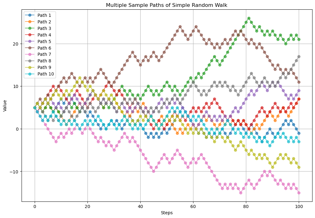
print(paths)

[[ 5  4  5 ...  1  0 -1]
 [ 5  4  5 ...  5  6  7]
 [ 5  6  5 ... 21 22 21]
 ...
 [ 5  6  5 ... 15 16 17]
 [ 5  6  5 ... -7 -8 -9]
 [ 5  4  3 ... -3 -2 -3]]

Exercise: Modeling Coffee Bean Prices with Random Walk

Coffee bean prices are known to fluctuate based on various market factors. Suppose we model the daily price of coffee beans using a random walk process with the following parameters:

• Probability of moving positively (\(p\)): \(0.6\)

• Initial price (\(a\)): \(100\) (hypothetical starting price in dollars)

• Size of increments: \(0.5\) (representing daily price fluctuations in dollars)

1. Define the random walk process for the daily price of coffee beans, \(X_n\).

2. Simulate and compute the price of coffee beans for the first 10 days.

3. Plot the simulated price path using Matplotlib.

Instructions:

• Implement the random walk process using Python.

• Display the simulated price path in a clear and readable format.

• Discuss the implications of the chosen parameters (\(p\), \(a\), increment size) on the volatility and trend of coffee bean prices.

• Use Monte Carlo methods to estimate the expected price at day 10 and estimate the probability that is greater than \(102\).

Solution: Modeling Coffee Bean Prices with Random Walk

1. Define the random walk process:

   Coffee bean price \(X_n\) is defined as:

   \[\begin{split} X_0 = 100 \\ X_n = X_{n-1} + Z_n \end{split}\]

where

\[\begin{split} Z_n = \begin{cases} 0.5, & \text{with probability } p \\ -0.5, & \text{with probability } 1 - p \end{cases} \end{split}\]

2. Simulate and compute the price for the first 10 days:

   Using Python, simulate the daily prices based on the defined process.

   import numpy as np
   import matplotlib.pyplot as plt
   
   np.random.seed(42)
   
   # Parameters
   n_days = 10
   p = 0.6
   increment = 0.5
   initial_price = 100
   
   # Generate random steps
   steps = np.random.choice([increment, -increment], size=n_days, p=[p, 1-p])
   
   # Compute price path
   price_path = np.cumsum(np.insert(steps, 0, 0)) + initial_price
   
   # Print the price path
   print(f"{'Day':<4} {'Price ($)':<10}")
   for day in range(n_days + 1):
       print(f"{day:<4} {price_path[day]:<10.2f}")
   
   # Plot the price path
   plt.figure(figsize=(10, 6))
   plt.plot(range(n_days + 1), price_path, marker='o', linestyle='-', color='b')
   plt.title('Daily Price of Coffee Beans')
   plt.xlabel('Day')
   plt.ylabel('Price ($)')
   plt.grid(True)
   plt.show()